(Takes a little while loading the images)
e-mail :

This document (Part XXIX Sequel-30) further elaborates on, and prepares for, the analogy between crystals and organisms.
Philosophical Context of the Crystal Analogy (VII)
In order to find the analogies that obtain between the Inorganic and the Organic (as such forming a generalized crystal analogy), it is necessary to analyse those general categories that will play a major role in the distinction between the Inorganic and the Organic : Process, Causality, Simultaneous Interdependency and the general natural Dynamical Law. This was done in earlier documents.
Sequel to the Categorical Analysis of 'Dynamical System ' and of Causality in terms of thermodynamics.
Why Thermodynamics plays such an important role in Nexus Categories.
The foregoing documents (Part XXIX Sequel-26, Sequel-27, Sequel-28 and Sequel-29) were about the general Categories of the Inorganic Category Layer (or Inorganic Layer of Being), such as Causality, Dynamical Law, Simultaneous Interdependency and Dynamical System. In these categories simultaneous, or through-time, nexus (plural) are involved, that is to say concretum-concretum determinations. For example, the Category of Causality, which is a nexus category, determines (which determination is a category-concretum determination) a certain type of concretum-concretum determination, i.e. determines a particular type of determination such that one concrete state determines another concrete state which (states) become thus connected to each other (i.e. they form a nexus), and in this way representing a particular type of nexus determination, and where this particular type of nexus determination is the concretum of the Category of Causality (Recall that a category is a principle that determines a 'concretum', which determination is a category-concretum determination, while a concretum-concretum determination is not a determination by a category, not a determination by a principle, but by a concrete entity on another concrete entity).
As has been said earlier, energy plays an important part in concretum-concretum determinations (and certainly not in category-concretum determinations, nor in category-category determinations), at least within the Inorganic Domain. It was, therefore, necessary to consider some elements of the 'science of heat' or thermodynamics, which is about energy conduction, energy conversion and energy dissipation, as they can be seen in physical and chemical processes. As a result, we now know more about the First, and, as importantly, about the Second Law of Thermodynamics, especially the latter's formulation in terms of entropy increase. It was mainly equilibrium thermodynamics which has been discussed, together with unstable dynamic systems. It leaded to a discussion of irreversibility and the possible probabilistic element in the nature of Causality.
But because we are intended to work out a comparison of crystals and organisms, and because organisms are far-from-equilibrium thermodynamic systems , we must now turn to the non-equilibrium thermodynamics and the associated dissipative systems and structures.
The most important source of these discussions are the two books of PRIGOGINE & STENGERS : Order out of Chaos, 1984 (1986), and Entre le temps et l'éternité, 1988 (Dutch edition, 1989). Further we will make use of Erich JANTSCH's book The Self-organizing Universe, 1980 (1987).
As a result, these discussions should shine some light on the nature of Causality as it is present in these dissipative systems and structures. At the same time, of course, the Category of Dynamical System itself will get analysed still better.
Non-equilibrium (or far-from-equilibrium) thermodynamic systems can produce order out of chaos. In spite of the (statistically) necessary overall increase of entropy, and thus overall increase of disorder, as a result of virtually any real-world process, these non-equilibrium systems can produce order, because they do that locally and then paying by entropy increase somewhere else. This means that such systems must be open : Matter and energy must be able to constantly enter the system, in order to keep it away from equilibrium, and matter and entropy must be allowed to leave the system. Of course, when we consider the environment, from which and to which matter, energy and entropy are transported, as belonging to the dynamic system, then this system is closed, its entropy, and thus its overall disorder, increases as a result of the running of the system. What is important is that these systems are (maintained) out of thermodynamic equilibrium.
The ordered structures they produce are called "dissipative structures", because energy is dissipated into their environment, which here means that entropy is exported from the structure into its environment. What we want to investigate here is whether crystallization, especially the formation of branched crystals (as we see them in snow and in windowpane frost) is such a dissipative system. We do this by investigating them thermodynamically. And if they indeed turn out to be dissipative systems (and their products -- crystals -- dissipative structures) we have obtained an important element of the crystal analogy, because all organisms are dissipative systems. To be a dissipative system is not something typically organic, because there are already many inorganic systems that definitely and certainly are dissipative dynamical systems (like, for instance, the well-known [but not yet totally understood] Belousov-Zhabotinsky Reaction).
On our Website (presently consisting of four Parts) we have already prepared for the study of dissipative non-equilibrium thermodynamic systems :
If necessary, the reader could consult these documents (again) in order to strenghen his or her understanding of the thermodynamics of crystal growth (especially branched crystals) and of (other) inorganic non-equilibrium systems (dissipative systems and structures).
In the course of the discussions about dissipative systems and structures we will try to determine whether at least the growth of branched crystals (dendritic crystals, stellar snow crystals, windowpane frost, etc.) allows to be characterized as representing a dissipative non-equilibrium thermodynamic process or system. In favor to this we could provisionally bring up the following :
But of course, if branched crystals are indeed demonstrated to be true dissipative structures, we only have demonstrated that branched crystals and organisms are thermodynamically identical. It still does not necessarily imply that organisms (and many non-strictly-crystalline inorganic dissipative structures for that matter) are some sort of crystals. That is to say we take our theory of organic lattices as still being unproven. And, as this theory already showed, organisms are certainly not "simply crystals", and even also not "simply branched crystals". They are much more sophisticated and regulated, and, moreover, historically evolved [long-range history], so they only can be, or represent, (branched) 'crystals' when the latter concept is substantially broadened. If we want to have an image in mind of an 'organic crystal', we should think of an organic version of a windowpane ice feather.
The next series of Figures [taken from Part XXIX Sequel-8 ] shows photographs of ordinary windowpane frost :


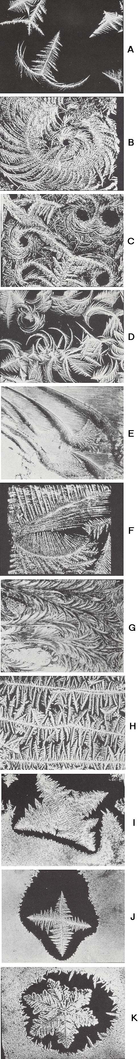
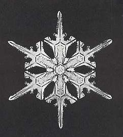
We can also think of an individual branch of a stellar snow crystal, as they are depicted in the next Two Figures (taken from Part XXIX Sequel-8) :
From the above photographs (and from all the others depicted in Part XXIX Sequel-8) it is clear that branched crystals possess a large morphological potential (and all these photographs refer to only one and the same substance, H2O, crystallized under normal conditions ! ).
Branched crystals of other substances can also have an 'organic look', like the metal silicides of the Figure HERE (also taken from Part XXIX Sequel-8 ) (close window to return to main text). When prepared by depositing the atoms from a vapor onto a cold surface, metal silicides such as (Cr,Fe)5Si3 crystallize into a variety of bizarre and dramatic shapes, as shown.
Probably we can say that branched crystals (as seen over their whole range) can generate any shape and structure imaginable.
When comparing branched crystals with organisms, it is perhaps productive to concentrate on (fast) molethynes , i.e. (forces in) directions of fast growth ( See Part XXIX Sequel-15 where we have discussed the molethynes [directional forces] in crystals), because molethynes occur both in crystals and in organisms. The connecting element for this is the Promorphology of organisms and of crystals. Promorphology investigates the global symmetry of an intrinsic object (organism, crystal) on the basis of the arrangement and number of its antimers (counterparts). The general theory of Promorphology, and its application to organisms can be found in the main Section "BASIC FORMS" (Promorphological System) in : Second Part of Website . The theoretic argument for the extension of Promorphology to crystals can also be found in Second Part of Website (at the end of it) at : "Basic Forms of Crystals" (especially Promorphology of Crystals I, II, and III ).
The Promorphology of crystals is further worked out in Part IV -- XXIX of present Part of Website. Much use have been made in these latter Parts (IV -- XXIX) of (imaginary) two-dimensional crystals, because they are easier to understand while at the same time illuminating most of the relevant general principles of shape, symmetry and promorph equally well as three-dimensional crystals can.
Although in crystals it is the periodic structure and the chemical and electrical properties of the potential faces that determine the differences in intrinsic growth rate and so determine the crystal's molethynes, it can be imagined that a periodic structure (characteristic for crystalline material) may not be a conditio sine qua non (i.e. an absolutely necessary [but not necessarily sufficient] reason or condition) for molethynes to be there. If this is so we can still compare organisms with crystals, even when organisms turn out to be in no way periodic, i.e. do not possess, even in a very hidden way, a periodic structure (that is to say, even when our theory of organic lattices turns out to be false).
What we have to do in what follows is to try to understand how it is possible that in real-world processes, although the global order must, as a result of these processes, decrease (net entropy increased, net leveling-out increased, as in heat conduction, where different temperatures in a given physical body are averaged), some of them can manage to effect a local increase of order (local decrease of entropy), as we see it in crystallzation and in many (non-equilibrium) dissipative systems. While the symmetry of a solution of some chemical substance (in a particular solvent) is maximal (every movement, reflection or rotation of the solution as a whole, returns the solution to its initial geometrical state), the symmetry of this solution + developing crystal has decreased as a result of crystallization, while it should in fact have stayed the same (because it cannot increase). It seems that in this consideration we cannot look macroscopically to the system (solution and crystal) but must do so microscopically. The heat (of fusion) given off by the developing crystal to the solution randomizes this solution still further (if we see this solution in terms of its many moving particles), while that part of the solution from which that heat is given off (the crystal) becomes less randomized than it was initially. If we compare the increase of randomization with the (local) decrease of it (as a result of the crystallization process), we must conclude, on the basis of the Second Law, that the amount of increase of randomization is larger than the amount of decrease, so that the netto randomization increases after all (despite the appearing of a crystal). But even seen in this (microscopic) way, it is remarkable that the system admits of local increase of order, because it then must have some 'overview' of the total situation.
Such cases lend themselves, therefore, to see all this from another (but compatible) viewpoint : Instead of focussing on the system-going-to-equilibrium as expressed by going to a state of maximum entropy -- which we do when also considering the environment, we can describe this going-to-equilibrium as going to a state of minimal free energy -- which we do when not considering the environment, which is equivalent to interpreting the system as an open system. So an open system, defined by boundary conditions such that its temperature T is kept constant (isothermal process) by heat exchange with the environment, equilibrium is not defined in terms of maximum entropy but in terms of the minimum of a similar function, free energy. The (amount of) free energy F is the (amount of) ordered (i.e. structured) energy, i.e. energy that can do work (causing volume changes for example), that is present in the system proper (that is, the system 'itself' without considering its environment). The free energy of the system proper is :
where E is the energy of the system (also, sometimes, denoted by U), and T the absolute temperature (See Part XXIX Sequel-18 ).
This formula signifies that equilibrium is the result of competition between energy and entropy. Temperature is what determines the relative weight of these two (physical) factors. At low temperatures, energy prevails, meaning that it is mainly the energy of the system that contributes to the system's free energy. And because at equilibrium the amount of free energy must be minimal, the amount of (just) energy is minimal. So it is here, that is, at low temperatures, that we find low-energy structures, such as crystals. Here, the entropy has decreased (because of the exhaust of heat to the environment). So crystals, that is to say equilibrium crystals, i.e. non-branched crystals, are low-energy, high-order, and weak-entropy structures.
At high temperatures, however, entropy is dominant : Also here the free energy must -- if the system is to go to equilibrium -- go to a minimum, and this will now be achieved by a high value of T, and therefore by a high value of TS, and therefore by a low value of ( E - TS ), and thus by a low value of F (whether the energy E is high or low, the high value of TS makes the value of F low. But because at high temperature it is entropy that dominates, we here get molecular disorder. The crystal melts.
The entropy S of an isolated system (or, equivalently, of an open system + its environment) and the free energy F of a system at fixed temperature (as it is the case in crystallization), and thus an open system (that as such is able to maintain a fixed temperature by importing or exporting heat from or to the environment), are examples of thermodynamic potentials. The extremes of thermodynamic potentials, i.e. of potentials such as S or F, define the attractor states toward which systems, whose boundary conditions (such as openess or isolation with respect to the environment) correspond to the definition of these potentials, tend spontaneously.
So in all these cases we have, in addition to a course towards a maximum of net entropy, to do with a course towards a minimum of free energy. But in true dissipative systems, like for instance organisms, the free energy has certainly not vanished or become very low, because we see that organisms are perfectly able to do work. So the difference between crystals and organisms is that the former have a minimum of free energy while the latter have a substantial amount of free energy at their disposal. But this is clear from the fact that crystals are equilibrium structures, and because of that have minimal free energy, while organisms are non-equilibrium structures (in fact far-from-(thermodynamic)-equilibrium structures), and are, therefore, not in a state of minimal free energy. As soon as they are in such a state they die.
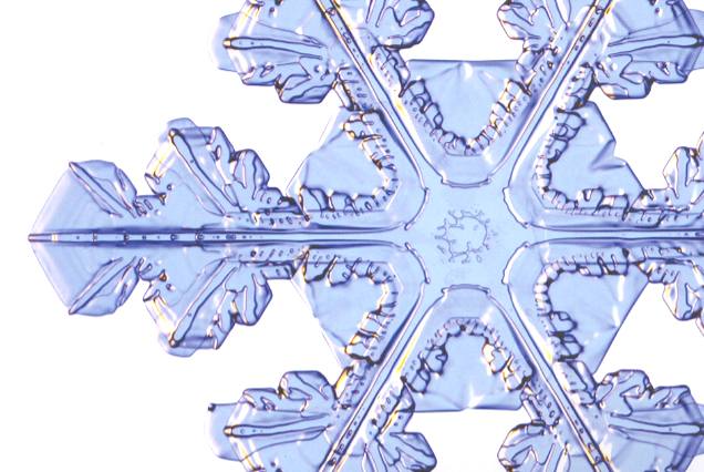
If, on the other hand, we turn to branched crystals (instead of ordinary crystals), the situation is different : Just like organisms, they are not equilibrium structures, and thus they are not in a state of minimal free energy. The particles of a branched crystal such as
(taken from Part XXIX Sequel-6) which is a (branched) snow crystal, still have the potential to move to other locations onto the crystal, to restore the 'true' hexagon-shaped crystal (without branches), as a crystal of the substance H2O should be. So we again and again see that it is branched crystals, or, generally, non-equilibrium crystals, that should play the role of crystals in the analogy between crystals and organisms.
It will be hard to determine the exact thermodynamic status (equilibrium thermodynamics, non-equilibrium linear thermodynamics, far-from-equilibrium non-linear thermodynamics) of the process that results in branched crystals, and whether they are, or are not, non-equilibrium stationary states, and what thermodynamic 'forces' (such as temperature gradients) might play a role in their formation and sustenance. Only with some answers to these questions can we decide whether branched crystals indeed can serve in the crystal analogy. And to come a little closer to these answers we must now discuss non-equilibrium thermodynamic systems, compare them with equilibrium systems, and differentiate between non-equilibrium linear and non-equilibrium non-linear thermodynamic systems. In all this we must make the transition from ideal system to real-world systems.
Entropy Flow and Entropy Production
There are reasons to distinguish between two ways that entropy can manifest itself : entropy flow, that is just transport of entropy, and entropy production, that is the very creation of entropy at a given location or in a given device.
But before we discuss this distinction we must repeat some relevant issues that were treated in the Section Thermodynamics of Part XXIX Sequel-28 , a document about the First and Second Laws of thermodynamics, about thermodynamic potentials such as entropy and free energy, about heat engines, heat pumps, thermal efficiency, etc.
There we found out that the thermal efficiency of a Carnot cycle , which is the most efficient type of ideal, reversible heat engine, is :
This means that even for a Carnot cycle the thermal efficiency is not perfect, i.e. not equal to 1 ( = 100 % ). This is because not all the imported heat can be transformed into work. Some must be exported, so Tc can never be equal to zero. But this efficiency is the highest possible of all reversible cycles operating between two fixed temperature extremes. So for any non-Carnot cycle the thermal efficiency is :
and this holds even more so for any irreversible cycle, because in such cycles heat is lost.
Also we found out that the thermal efficiency of any (ideal) heat engine is :
So the efficiency of any engine (not any other engine, but any (ideal) engine whatsoever, thus including a Carnot cycle) is
or rewritten
The equality sign (as it is present in  and
and  ) takes the fact into account that such an engine might be a Carnot cycle.
In analysing a(n ideal) heat engine for each complete cycle the total change in the entropy of the entire system was accounted for (in the Section Entropy and the Second Law of Thermodynamics ) as follows :
So for any system (inclusing a possible Carnot cycle) we have for the entropy change  the following :
and if we exclude the Carnot cycle we have :
That is to say, for any, even ideal, but non-Carnot engine the entropy of the entire system always increases.
REMARK :
So for such r e v e r s i b l e engines there must -- according to the above -- be an entropy i n c r e a s e , despite the assertion by WEIDNER, Physics, 1989, p.484, that in the expression
Anyway,
 is the efficiency of any (ideal) engine (where "ideal" always means : without friction and the like ) , so also of a Carnot engine. Thus, if we express the efficiency of a Carnot engine by Qc and Qh then we have :
and thus, according to the finding
we have for the Carnot cycle :
That is to say, that in the Carnot cycle the net entropy does not change, or, equivalently, the net exported reduced heat is zero. Especially important is the fact that in any spontaneous process, including the (ideal) Carnot process, the entropy cannot decrease (which is what the Second Law of Thermodynamics expresses). "Spontaneous" here means that the process is not forced to stay away from (thermodynamic) equilibrium. In all other ideal engines the net entropy increases.
And of course it is clear that all real-world engines or processes (where there is friction, heat losses, and the like) do increase the net entropy.
The fact that even already in the case of the (ideal and reversible) Carnot engine the efficiency is lower than 100 % (i.e. smaller than 1), expresses a fundamental fact (instead of just expressing friction, heat losses [the whole machine gets warm], and the like), the fact namely that even in an ideal heat engine not all supplied heat can be converted to work.
And this is in fact what is said by the Second Law of Thermodynamics.
In the document about Thermodynamics (Part XXIX Sequel-28) we came across three equivalent formulations of the Second Law, and it is useful to give them here again :
Now we are ready to discuss the above mentioned two ways in which entropy can manifest itself (and which distinction plays a role in characterizing the three types or stages of thermodynamic systems : Equilibrium thermodynamic systems, non-equilibrium linear thermodynamic systems, and non-equilibrium non-linear thermodynamic systems [truly dissipative systems] ) : Entropy flow and Entropy production. This distinction makes sense as soon as we consider real-world thermodynamic systems.
Let us (following PRIGOGINE & STENGERS, Order out of Chaos, pp.118 of the 1986 Flamingo edition) consider the variation of the entropy, dS, over a short time interval dt. The situation is quite different for ideal and real engines. In the first case, dS may be expressed completely in terms of the exchanges between the engine and its environment. We can set up experiments in which heat is given up by the system instead of flowing into the system. The corresponding change in entropy would simply have its sign changed. This kind of contribution to entropy, which we shall call deS , is therefore reversible in the sense that it can have either a positive or a negative sign. The situation is drastically different in a real engine. Here, in addition to reversible exchanges, we have irreversible processes inside the system, such as heat losses, friction, and so on. These produce an entropy increase or "entropy production" inside the system. The increase of entropy, which we shall call diS , cannot change its sign through a reversal of the heat exchange with the outside world. Like all irreversible processes (such as heat conduction), entropy production always proceeds in the same direction. The variation is monotonous : entropy production cannot change its sign as time goes on.
The notations deS and diS have been chosen to remind the reader that the first term refers to exchanges (e) with the outside world, that is, with entropy flow, while the second refers to the irreversible processes inside (i) the system, that is, with entropy production.
The entropy variation dS is therefore the sum of the two terms deS and diS , which have quite different physical meanings.
To grasp the peculiar feature of this decomposition of entropy variation into two parts, it is useful first to apply it to something to which it cannot be meaningfully applied, for instance to energy, and then to apply it to something else than entropy variation where it can be applied meaningfully, namely, for instance, the quantity of hydrogen in some given container.
So let us apply an analogous decomposition to energy, and let us denote energy by E and variation over a short time dt by dE. Of course, we would still write that dE is equal to the sum of a term deE due to the exchanges of energy, and a term diE linked to the "internal production" of energy. However, the principle of conservation of energy states that energy is never "produced" but only transferred from one place to another. The variation in energy dE is then reduced to deE . And because this is always so, the decomposition of dE into the two terms mentioned is not very useful.
On the other hand, if we take a non-conserved quantity, such as the quantity of hydrogen molecules contained in a vessel, this quantity may vary both as a result of adding hydrogen to the vessel (hydrogen flow into the system), or through chemical reactions occurring inside the vessel. But in this case, the sign of the "production" is not determined (as it is in entropy production). Depending on the circumstances, we can produce or destroy hydrogen molecules by detaching hydrogen from compounds that were in the vessel or by letting hydrogen being taken up in some compound by a chemical reaction.
The peculiar feature of the Second Law is the fact that the production term diS is always positive. The production of entropy expresses the occurrence of irreversible changes inside the system. If we leave the Carnot cycle and consider other thermodynamic systems, the distinction between entropy flow and entropy production can still be made. For an isolated system that has no exchanges with its environment, the entropy flow is, by definition, zero. Only the production term remains, and the system's entropy can only increase or remain constant. Increasing entropy corresponds to the spontaneous evolution of the system. Increasing entropy is no longer synonymous with loss, but now refers to the natural processes within the system. These are the processes that ultimately lead the system to thermodynamic equilibrium corresponding to the state of maximum entropy.
Reversible transformations belong to classical science in the sense that they define the possibility of acting on a system, of controlling it. The (purely) dynamic object could be controlled through its initial conditions. Similarly, when defined in terms of its reversible transformations (that is, considering the [thermodynamic] system as being ideal, meaning no friction and the like), the thermodynamic object may be controlled through its boundary conditions ( These are about the system's relations to its environment -- such as ambient temperature, insulatedness or openess, the system being maintained in a certain volume and under a certain pressure -- and so determine the relevant thermodynamic potential -- entropy, free energy, or other such potentials -- and with it the latter's extreme [maximum entropy, minimum free energy, and the like] and consequently determine the system's attractor ) :
Any system in thermodynamic equilibrium whose temperature, volume, or pressure are g r a d u a l l y changed, passes throug a series of equilibrium states (PRIGOGINE & STENGERS, Ibid. p.120),
and any reversal of the manipulation leads to a return to its initial state. The (defined) reversible nature of such change and controlling the object through its boundary conditions are interdependent processes. In this context irreversibility is "negative". It appears in the form of "uncontrolled" changes that occur as soon as the system eludes control. But inversely, irreversible processes may be considered as the last remnants of the spontaneous and intrinsic activity displayed by nature when experimental devices are employed to harness it.
Thus the "negative" property of dissipation shows that, unlike purely dynamic objects, thermodynamic objects can only be partially controlled. Occasionaly they "break loose" into spontaneous change.
For a thermodynamic system not every change is equivalent to every other change . This is the meaning of the expression
Spontaneous change diS toward equilibrium is different from the change deS , which is determined and controlled by a modification of the boundary conditions (for example, ambient temperature).
For an isolated system, equilibrium appears as an "attractor" of non-equilibrium states. (PRIGOGINE & STENGERS, Ibid. p.120).
The initial assertion (all changes are not equivalent) may thus be generalized by saying that evolution toward an attractor state (involving diS ) differs from all other changes, especially from changes determined by boundary conditions (and thus involving deS ).
Max Planck (as PRIGOGINE & STENGERS report) often emphasized the difference between the two types of change found in nature. Nature, wrote Planck, seems to "favor" certain states. The irreversible increase in entropy diS / dt (entropy change in time) describes a system's approach to a state which "attracts" it, which the system prefers and from which it will not move volontarily.
"From this point of view, Nature does not permit processes whose final states she finds less attractive than their initial states. Reversible processes are limiting cases. In them, Nature has an equal propensity for initial and final states. This is why the passage between them can be made in both directions." (quoted by PRIGOGINE & STENGERS).
How foreign such language sounds when compared with the language of dynamics ! (say PRIGOGINE & STENGERS). In dynamics, a system changes according to a trajectory that is given once and for all, whose starting point is never forgotten (since initial conditions determine the trajectory for all time). However, in an isolated thermodynamic system all non-equilibrium situations produce evolution toward the same kind of equilibrium state. By the time equilibrium has been reached, the system has forgotten its initial conditions -- that is, the way it had been prepared.
Thus, say, specific heat or the compressibility of a system in equilibrium are properties independent of the way the system has been set up. This fortunate circumstance greatly simplifies the study of the physical states of matter. Indeed, complex systems consist of an immense number of particles. From the dynamic standpoint it is, in the case of systems with many particles, practically impossible to reproduce any state of such systems in view of the infinite variety of dynamic states that may occur. Were knowledge of the system's history indispensable for understanding the mentioned properties, we would hardly be able to study them.
We are now confronted with two basically different descriptions : dynamics, which applies to the world of motion, and thermodynamics, the science of complex systems with its intrinsic direction of evolution toward increasing entropy. This dichotomy immediately raises the question of how these descriptions are related, a problem that has been debated since the laws of thermodynamics were formulated. It is the question, thus, of how the formulations of thermodynamics can be reconciled with those of dynamics. We will find a direction to its answer in the order principle of Boltzmann. We have discussed this principle in the Section "Microscopic consideration of entropy" in Part XXIX Sequel-28 . Boltzmann's results signify that irreversible thermodynamic change is a change toward states of increasing probability and that the attractor state is a macroscopic state corresponding to maximum probability ( that is, not a particular individual state, but a category or type of states (as such macroscopically recognizable, as a category of distribution [of places, velocities, and so on] ) ). The category with the highest number of complexions ( = number of permutations or number of ways such a category can be (theoretically) achieved, and giving the relative probability of such a category to be realized ) has the highest probability to represent the state of the system.
The distribution category corresponds to a macroscopic state, whereas an individual distribution (i.e. any particular distribution) corresponds to a microscopic state.
All this takes us far beyond Newton. For the first time a physical concept has been explained in terms of probability. Its utility is immediately apparent. Probability can adequately explain a system's forgetting of all initial dissymmetry (that is, low symmetry), of all special distributions (for example, the set of particles concentrated in a subregion of the system [and later to diffuse all over the system], or the distribution of velocities that is created when two gases of different temperatures are mixed [and which (dissymmetric) distribution will eventually become homogenized] ). This forgetting is possible because, whatever the evolution peculiar to the system, it will ultimately lead to one of the microscopic states corresponding to the macroscopic state (distribution category) of disorder and maximum symmetry (that is, homogeneity), since such a macroscopic state corresponds to the overwhelming majority of possible microscopic states (that is to say, such a macroscopic state can, as a category, be achieved in an enormous number of different ways, where each way represents an individual distribution pertaining to that category). Once this state has been reached, the system will move only short distances from the state, and for short periods of time. In other words, the system will merely fluctuate around the attractor state.
Boltzmann's order principle implies that the most probable state available to the system is the one in which the multitude of events taking place simultaneously in the system compensates for one another statistically. In the case of a gas, initially present in only one half of a container, or, whatever the initial distribution of it over the two halves of the container was, the system's evolution will ultimately lead it to the equal distribution N1 = N2 (number of particles in the left half equals the number in the right half of the container). This state will put an end to the system's irreversible macroscopic evolution. Of course, the particles will go on moving from one half to the other, but on the average, at any given instant, as many will be going in one direction as in the other. And this is just the same as to say that the many possible individual distributions belonging to the distribution category characterized by the presence of (just) equal numbers of particles in the two halves of the container, alternate among one another. As a result, the motion of the particles will cause only small, short-lived fluctuations around the equilibrium state N1 = N2 . Boltzmann's probabilistic interpretation thus makes it possible to understand the specificity of the attractor studied by equilibrium thermodynamics.
Let us now proceed our course toward non-equilibrium thermodynamics.
In the kinetics involved in thermodynamic processes we must consider the rates of irreversible processes such as heat transfer and the diffusion of matter. The rates (we could say the speed) of irreversible processes are also called fluxes and are denoted by the symbol J . The thermodynamics of irreversible processes introduces a second type of quantity : in addition to the rates, or fluxes, J , it uses "generalized forces", X , that "cause" the fluxes. The simplest example is that of heat conduction. Fourier's law tells us that the heat flux J is proportional to the temperature gradient. This temperature gradient is the "force" causing the heat flux. By definition, flux and forces both vanish at thermal equilibrium. The production of entropy P = diS/dt can be calculated from the flux and the forces.
As could be expected, all irreversible processes have their share in entropy production. Each process participates in this production through the product of its rate or flux J multiplied by the corresponding force X. The total entropy production per unit time (i.e. the rate of change of entropy in time), P = diS/dt , is the sum of these contributions. Each of them appears through the product JX.
We can divide Thermodynamics into three large fields, the study of which corresponds to three successive stages in its development :
Entropy production, the fluxes, and the forces are all zero at equilibrium.
In the close-to-equilibrium region, where thermodynamic forces are "weak", the rates Jk are linear functions of the forces.
The third field is called the "non-linear" region, since in it the rates are in general more complicated functions of the forces.
Let us first emphasize some general features of linear thermodynamics that (therefore) apply to close-to-equilibrium situations. We'll do this by means of an instructive example, thermodiffusion. See next Figure.
We have two closed vessels connected by a tube, and filled with a mixture of two different gasses, for example hydrogen and oxygen. We start with an equilibrium situation : The two vessels have the same temperature and pressure and contain the same homogeneous gas mixture. Now we apply a temperature difference Th --- Tc between the two vessels. The deviation from equilibrium as a result of this temperature difference can only be maintained when the temperature difference is maintained (because if we do nothing, the whole system will end up with the same temperature all over again (lying between the two initial temperatures) as a result of heat conduction, that is, the system ends up at equilibrium again). So we need a constant heat flux which compensates the effects of thermal diffusion : one vessel is constantly heated (Qh in), while the other is cooled (Qc out). So the system is constantly subjected to a thermodynamic force, namely the thermal gradient. The experiment shows that, in connection with the thermal diffusion (heat conduction from one vessel to the other) a process appears in which the two gasses become separated. When the system has reached its stationary state in which at a given heat flux in and out of the system the temperature difference remains the same as time goes on, then more hydrogen will be present in the warmer vessel and more oxygen in the cold vessel. That is to say, a concentration gradient is the result. The difference in concentration (i.e. the degree of separation) is proportional to the temperature difference. So the thermodynamic force, which here was the temperature gradient, has effected a concentration gradient, where initially the concentration was uniform. As long as the temperature difference is maintained, the separation will be maintained. In fact (according to PRIGOGINE, 1980, p.87) the system has two forces, namely Xk , corresponding to the difference in temperature between the two vessels, and Xm corresponding to the chemical potential [which I presume to be, in the present case, the concentration gradient] between the two vessels, and (the system has) two corresponding flows (fluxes), Jk (heat flow), and Jm (matter flow). The system reaches a state in which the transport of matter vanishes, whereas the transport of energy between the two phases (vessels) at different temperatures continues, that is, a steady non-equilibrium state. Such a state should not be confused with an equilibrium state characterized by a zero entropy production.
It cannot be denied that the transformation from a homogeneous distribution of the two gasses to a separation of them means an increase in the order of the system. But this is so because the system is open, and is constantly being subjected to the mentioned thermodynamic force. And as long as this force (temperature gradient) is moderate, it will be proportional to its effect (concentration gradient), that is to say, the system is then linear (or, equivalently, it finds itself in the linear region) : When the force is doubled, so is its effect, when it is tripled, so its effect, and so on.
We see that in this case the activity which produces entropy (the diffusion of heat all over the system) cannot simply be identified by the leveling out of differences. Surely, the heat flux from one vessel to the other plays this role, but the process of separation of the two gasses that originates by virtue of the coupling with the thermal diffusion (within the system) is itself a process by which a difference is created, an 'anti-diffusion' process which provides a negative contribution to the entropy production. This simple example of thermodiffusion shows how important it is to abandon the idea that activity in which entropy is produced (heat diffusion within the system) is equivalent to degradation, that is, with the leveling out of differences. For although it is true, that we have to pay an entropy fee for the maintenance of the stationary state of the thermodiffusion process, it is also true that that state corresponds with the creation of order. In such a non-equilibrium thermodynamic process a new view is possible : We can evaluate the disorder that has originated as a result of the maintenance of the stationary state as that which makes possible the creation of a form of order, namely a difference in chemical composition in the two vessels. Order and disorder are here not opposed to each other but are inextricably connected. The next Figure shows how it is with the entropy fee : In order to maintain the temperature difference (and thus to maintain the system's stationary state of separated gasses) the (relevant part of the) environment, which initially enjoyed some (temperature) difference looses this difference.
Figure above : Thermodiffusion : The entropy fee, payed by the environment to create (local) order.
The thermodiffusion process reminds us a little of the Carnot process , discussed in Part XXIX Sequel-28, but it is in fact quite different, despite the fact that both involve a permanent difference which is, so to say, the motor of the production of order (that is, work in the Carnot process, and chemical separation in the thermodiffusion process), like a difference in water level can drive a turbine.
The Carnot process has the following properties :
Linear (non-equilibrium) thermodynamics of irreversible processes is dominated by two important results, namely the Onsager reciprocity relations and the theorem of minimal entropy production.
Let us first discuss the Onsager reciprocity relations.
In 1931, Lars Onsager discovered the first general relations in non-equilibrium thermodynamics for the linear, near-to-equilibrium region. We will explain (not prove) these relations by using the just discussed thermodiffusion experiment.
This experiment in fact consists of two processes, which we shall call
Process 1 and Process 2 :
Figure above : The two processes, 1 and 2, the two forces, 1 and 2, an the two fluxes 1 and 2, in the thermodiffusion experiment.
With the help of the above Figure we can now state the Onsager relations :
When the Flux 1, corresponding to the irreversible Process 1, is influenced by the Force 2 of the irreversible Process 2, then the Flux 2 is also influenced by the Force 1 through the same coefficient L12 , that is, L12 = L21 ( PRIGOGINE, From Being to Becoming, 1980, p.86 ).
This holds for all linear non-equilibrium systems, for example, in each case where a thermal gradient induces a process of diffusion of matter, we find that an applied concentration gradient to that system can set up a heat flux through the system.
The importance of the Onsager relations resides in their generality. They have been submitted to many experimental tests. Their validity showed, for the first time, that non-equilibrium thermodynamics leads, as does equilibrium thermodynamics, to general results independent of any specific molecular model. It is immaterial, for instance, whether the irreversible processes take place in a gaseous, liquid, or solid medium. This is the feature that makes the Onsager relations a thermodynamic result.
What follows now is taken (not necessarily as a quote) from PRIGOGINE & STENGERS, Order out of Chaos, pp.138 of the 1986 Flamingo Edition (with some comments of mine between square brackets).
Reciprocity relations have been the first results in the thermodynamics of irreversible processes to indicate that this was not some ill-defined no-man's land, but a worthwhile subject of study whose fertility could be compared with that of equilibrium thermodynamics. Equilibrium thermodynamics was an achievement of the nineteenth century, non-equilibrium thermodynamics was developed in the twentieth century, and Onsager's relations mark a crucial point in the shift of interest away from equilibrium thermodynamics toward non-equilibrium thermodynamics.
A second general result in this field of linear, non-equilibrium thermodynamics is that of mimimal entropy production. We have already spoken of thermodynamic potentials whose extrema correspond to the states of equilibrium toward which thermodynamic evolution tends irreversibly (such as the leveling out of temperature by heat conduction). Such are the entropy S for isolated systems, and the free energy F for open systems at a given temperature (that is, at a constant temperature). The thermodynamics of close-to-equilibrium systems also introduces such a potential function. It is quite remarkable that this potential is the entropy-production P itself. The theorem of minimum entropy production does, in fact, show that in the range of validity of Onsager's relations -- that is, the linear region -- a system evolves toward a stationary state characterized by the minimum entropy production (which is thus the extreme of the entropy production potential) compatible withe constraints imposed upon the system. These constraints are determined by the boundary conditions. They may, for instance, correspond to two points in the system kept at different temperatures, or to a flux of matter that continuously supports a reaction and eliminates [i.e. exports] its products.
The stationary state toward which the system evolves is then necessarily a non-equilibrium state at which dissipative processes with non-vanishing rates occur. But since it is a stationary state, all the quantities that describe the system, such as temperature, concentrations, and so on, become time-independent. Similarly, the entropy of the system now becomes independent of time. Therefore its time variation vanishes, dS = 0.
But we have seen above that the time variation of entropy is made up of two terms -- the entropy flow deS and the positive entropy production diS . Therefore, dS = 0 implies that deS = -diS < 0 (that is, because diS is positive, and dS = deS + diS = 0, deS must be the same in absolute value as is diS but with opposite sign). The heat or matter flux coming from the environment determines a negative flow of entropy deS , which is, however, matched by the entropy production diS due to irreversible processes inside the system. A negative flux deS means that the system transfers entropy to the outside world. Therefore at the stationary state, the system's activity continuously increases the entropy of its environment [See Figure farther above ]. This is true for all stationary states. But the theorem of minimum entropy production says more. The particular stationary state toward which the system tends is the one in which this transfer of entropy to the environment is as small as is compatible with the imposed boundary conditions. In this context, the equilibrium state corresponds to the special case that occurs when the boundary conditions allow a vanishing entropy production. In other words, the theory of minimum entropy production expresses a kind of 'inertia'. When the boundary conditions prevent the system from going to equilibrium it does the next best thing. It goes to a state of minimum entropy production -- that is, to a state as close to equilibrium as 'possible'.
Linear thermodynamics thus describes processes that spontaneously tend toward the extreme of some thermodynamic potential, which potential here is entropy production while its extreme is minimal entropy production, and therefore the stationary state is, like the equilibrium state of equilibrium thermodynamics, stable. So linear thermodynamics describes the stable, predictable behavior of systems tending toward the minimum level of activity compatible with the fluxes that feed them. The fact that linear thermodynamics, like equilibrium thermodynamics, may be described in terms of a potential, the entropy production, implies that, both in evolution toward equilibrium and in evolution toward a stationary state, initial conditions are forgotten. Whatever the initial conditions, the system will finally reach the state determined by the imposed boundary conditions (which in turn determine the kind of relevant thermodynamic potential). As a result, the response of such a system to any change in its boundary conditions (for example (not too high) an increase of the applied difference of temperature) is entirely predictable.
We see that in the linear range (that is, close to equilibrium) the situation remains basically the same as at equilibrium. Although the entropy production does not vanish (as it does at equilibrium), neither does it prevent the irreversible change from being identified as an evolution toward a state that is wholly deducible from general laws. This 'becoming' inescapably leads to the destruction of any difference, any specificity [ That is to say, just like in equilibrium thermodynamics, from whatever initial condition, possessing whatever differences and specificities, the system leaves it all behind and evolves toward a general attractor state determined by the extremum of its thermodynamic potential ]. Carnot or Darwin? The question remains. There is still no connection between the appearance of natural organized forms on one side, and on the other the tendency toward 'forgetting' of initial conditions, along with the resulting disorganization (PRIGOGINE & STENGERS, Ibid., p.140) [ One should not forget, however, that in close-to-equilibrium systems local order can appear, as seen in thermodiffusion. But the stationary state is, like the equilibrium state, stable and predictable, and thus has no potential to 'venture into new territory' ]. As we will see, all that changes, when the system is driven far-from-equilibrium, and as a result enters the non-linear domain.
Crystallization
After having discussed general equilibrium thermodynamics (in Part XXIX Sequel-28 ) (inserted in the discussion of models of unstable systems, in order to have a good understanding of entropy and energy), and (after having discussed) general close-to-equilibrium thermodynamics (present document), it is now time to discuss, at least in a preliminary way, the thermodynamic status of plain crystallization (i.e. the formation of plain crystals, not of branched crystals). It is not easy to assess this status, even after having considered so much general thermodynamics. So the following discussuion is -- especially because the author of this website is not a professional physicist or chemist -- is indeed only preliminary and not in all respects certain of free of inconsistencies.
Crystals can appear either in solution or in a melt, or directly from a vapor.
Like in thermodiffusion (which is a close-to-equilibrium process), in crystallization local order emerges as a result of an imposed fall, that is of an imposed difference, which is as such a thermodynamic force, and which causes a flux of some kind (and where the force and the flux are supposed to be linearly related).
In the case of thermodiffusion the imposed force is a difference in temperature. And this force is applied to an initially homogeneous system, that is, a system in which two gases are uniformly distributed over the system. As a result of the application of the force the uniform distribution of the gases becomes unstable, the gases separate and (thus) local order emerges. This order endures as long as the force is applied. Entropy is given off to the environment, and as long as the force is not too great, that is, as long as the system remains linear, the entropy production and its transfer to the environment will be minimal, i.e. it will be as low as the boundary conditions permit. When the force is no longer applied, the system becomes an equilibrium thermodynamic system : The temperature becomes uniform, the force is zero and so are the fluxes that were (ultimately) caused by it. The separation of the two gases will become undone.
In order to induce (plain) crystallization from a solution we must impose a force of concentration : The solution must be moderately supersaturated. Here then we have created a fall : supersaturation -- saturation. When a solution is made supersaturated with respect to some solute, it means that the solution, that is the uniform distribution of the solute in the solvent, becomes unstable. Above a certain size, a crystal 'embryo', that had emerged by chance in the solution, will lower the free energy when it grows larger, so it will spontaneously grow larger. So a crystal is growing in the solution. And if the supersaturation level is maintained (for instance by letting the solvent slowly evaporate during crystallization), the crystal will keep on growing. As long as this is the case we have, I think, to do with a close-to-equilibrium system. In contrast to equilibrium systems it creates local order. The growing crystal is never in complete equilibrium because of the ever-present surface energy (caused by dangling chemical valences, or distorted or disconnected bonds), and as long as the mentioned level of difference is kept, the growing crystal exports entropy to the environment, randomizing this environment instead of itself.
For crystallization directly from a vapor (as it (always) occurs, for instance, in the case of snow crystal formation) (See Part XXIX Sequel-13 about phase transitions) , the imposed fall also consists of a distance, here in fact of two distances (differences), namely (1) the distance between (moderate) supersaturation and saturation or even undersaturation ( In the case of snow, very high levels of supersaturation, that is, very high humidities, can result in branched crystals, whereas moderate or low humidities (moderate or low supersaturation of air with water vapor, or even undersaturation) generally create plain stable crystals having the form of hexagonal prisms ), and (2) a distance (difference) in temperature (supercooling-temperature -- melting point temperature). Also here order is created and entropy is exported to the environment.
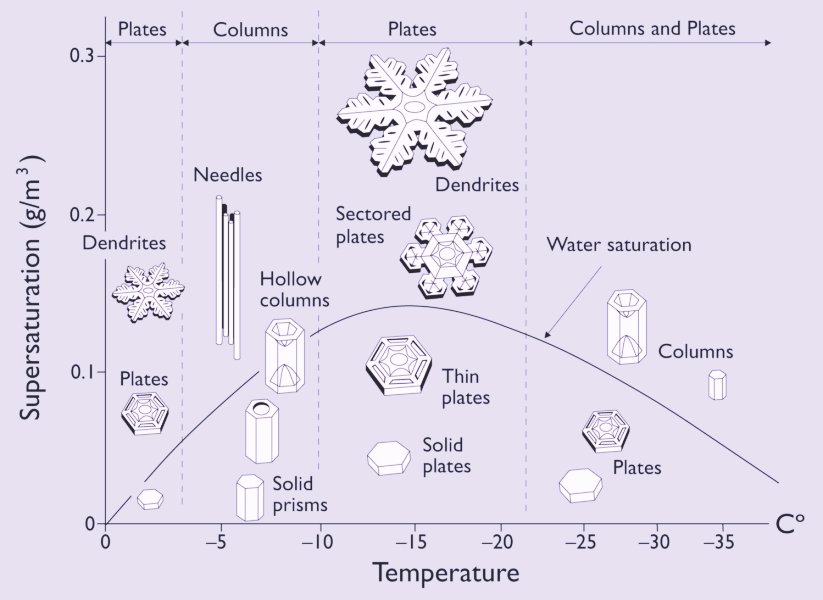
For snow crystals, which always originate directly from water vapor in the air, one has constructed a morphology diagram that displays the forms of snow crystals as a function of humidity (undersaturation -- supersaturation) and ambient temperature. The curved line in it is the water saturation line. It gives the humidity for air containing water droplets, as might be found within a dense cloud. That is to say it indicates the saturation of air with water vapor as a function of air temperature. The diagram can be inspected HERE .
For crystallization from a melt (See Part XXIX Sequel-13 about phase transitions) the imposed difference is that of temperature (supercooling-temperature -- melting point). As long as supercooling is maintained and is moderate, plain crystals will appear (from embryos) as a result, because under these conditions the melt is unstable. Heat will be given off by the crystallization process locally increasing the temperature up to the melting point, and, in addition randomizing the environment. Crystallization from a melt is discussed in Part XXIX Sequel-14 , and basing myself on that discussion, we can add the following with respect to crystallization from a melt and its thermodynamic status (where DELTA Gv is the difference between the free energy of formation of the crystal and that of the melt, times the volume of the crystal, (and where) DELTA Gs is the total surface energy, (and where) DELTA G = DELTA Gv + DELTA Gs , and where stable configurations are those with lowest free energy) :
If the (boundary) conditions (temperature and pressure) are such that DELTA G < 0 (G is decreasing while the crystal grows), which means that the degree of being negative of DELTA Gv is such that even when DELTA Gs is added, DELTA G is still negative, then a given crystal embryo above a certain size will grow (instead of disintegrate again), i.e. a crystal is growing in the melt. Heat of fusion is given off to the melt, but as long as there is supercooling in such a degree that the surface energy DELTA Gs (which appears as soon as there appears a crystal) is overcome (by the stronger degree of being negative of DELTA Gv at those supercooling-temperatures), the crystal keeps on growing. This means that a state of non-equilibrium (supercooling) is necessary for the crystal to grow, that is, the fall (i.e. the difference) between the melting point and the supercooling temperature is necessary.
At equilibrium, on the other hand, that is when the temperature is exactly at the melting point (no supercooling), crystallization does not get off the ground. The melt and crystalline states have then exactly the same energy, DELTA Gv = 0 and thus DELTA G > 0 because of the surface energy. While embryos may form by chance, the surface energy ensures that DELTA G of crystal growth is positive for all embryo sizes. All crystal embryos, regardless of size, are therefore unstable with respect to the melt and will be destroyed.
The fact that crystals do not beginforming as soon as the temperature drops slightly below the equilibrium temperature (the melting or freezing point) indicates that melt is remaining metastable with respect to crystals. To get crystals growing, it is necessary to supercool the melt to provide the activation energy (needed to knock the metastable state over the balance) to overcome the difficulties related to surface energy (NESSE, W. Introduction to Mineralogy, 2000, p.78).
So supercooling, with respect to crystallization in a melt, is necessary to keep the crystal growing, because its total surface energy is increasing as the crystal grows (Surface energy : The disrupted chemical bonds at the surface of each crystal, or crystal embryo, represent a higher energy configuration. The magnitude of the surface energy is proportional to the surface area ). Therefore crystallization (here shown for crystallization from a melt) is a non-equilibrium process (It is kept from equilibrium, that is, as long as it is kept from equilibrium).
The considerations about crystallization from a melt, as presented here, are, after having made the appropriate changes, also valid for crystallization from a solution (Here the fall to be maintained is the degree of supersaturation).
For plain crystallization in general (from solution, vapor or melt) and for the comparison with other processes, we can further say : Apart from friction and heat losses, in a real Carnot engine there is no dissipation involved in this engine (because of the thermal insulation of the hot source from the cold), meaning that there is no intrinsic dissipation. Therefore an ideal Carnot engine is reversible. On the other hand, in crystallization there is intrinsic dissipation : the released heat of fusion (which {further} randomizes the environment).
So crystallization is an intrinsically irreversible process. But this does not already make crystallization a non-equilibrium process (that is, a process held away from equilibrium), because just the process of ordinary heat conduction in some material, leveling out temperature differences, is an irreversible process that nevertheless goes to equilibrium.
With the concept " i r r e v e r s i b l e" we do not mean that a given process type cannot have two possible directions (direct and reverse). What we mean is that an individual process as it has just happened, and if it can be called irreversible, cannot retrace its foot steps. In this way heat dissipation is irreversible. If it were reversible, then every atom or molecule that was involved in the handing-over of kinetic energy (leading to the leveling out of temperature) would undo what it had done, in order for the system to arrive at the initial condition again, along the same way along which it initially departed from that initial condition. This is highly improbable to say the least.
So crystallization is intrinsically irreversible, but it represents a non-equilibrium process only in combination with the fact that a constant fall (that is, some thermodynamic force) is applied (or, as long as this fall is applied) to the system.
We do not know whether the theorem of minimum entropy production applies for (plain) crystallization. Certainly a definite amount of heat is given off to the environment : Upon melting, solving, or vaporizing, heat is imported to randomize the disintegrating crystal. When, on the other hand, the crystal is generated, this heat is given off again. And because during crystallization there is a well-defined temperature, we can say that a definite amount of entropy is exported to the environment. This to be a minimum entropy production, seems likely.
So in all, it is pretty clear that plain crystallization is not an equilibrium process (in which only a leveling-out is created, not (local) order), but a close-to-equilibrium process (in which, as in thermodiffusion, (local) order is created). And as long as the imposed fall (the imposed thermodynamic force) is moderate the corresponding fluxes are proportional to this force and the system is linear. This will change dramatically in the case of branched crystals, where the imposed force (very high humidity in the case of snow crystals) is very strong.
In all equilibrium processes the end state is stable. And in close-to-equilibrium processes the stationary state (growing crystal, separation of gases) is also a stable state, as it should be in linear systems.
Far from Equilibrium (PRIGOGINE & STENGERS, Ibid., pp.140).
At the root of non-linear thermodynamics lies somthing quite surprising, something that first appeared to be a failure : In spite of much effort, the generalization of the theorem of minimum entropy production for systems in which the fluxes are no longer linear functions of the forces appeared impossible. Far from equilibrium [that is, when the applied fall is great], the system may still evolve to some steady state, but in general this state can no longer be characterized in terms of some suitably chosen potential (such as entropy production for near-equilibrium states).
The absence of any potential function raises a new question
: What can we say about the stability of the states toward which the system evolves? Indeed, as long as the attractor state is defined by the minimum of a potential such as the entropy production, its stability is guaranteed. It is true that a fluctuation may shift the system away from this minimum. The second law of thermodynamics, however, imposes the return toward the attractor. The system is thus 'immune' with respect to fluctuations. Thus whenever we define a potential, we are describing a "stable world" in which systems follow an evolution that leads them to a static situation that is established once and for all.
When the thermodynamic forces acting on a system become such that the linear region is exceeded, however, the stability of the stationary state, or its independence from fluctuations, can no longer be taken for granted. Stability is no longer the consequence of the general laws of physics. We must examine the way a stationary state reacts to the different types of fluctuation produced by the system or its environment. In some cases, the analysis leads to the conclusion that a state is "unstable" -- in such a state, certain fluctuations, instead of regressing, may be amplified and invade the entire system, compelling it to evolve toward a new regime that may be qualitatively quite different from the stationary states corresponding to minimum entropy production.
Thermodynamics leads to an initial general conclusion concerning systems that are liable to escape the type of order governing equilibrium. These systems have to be "far from equilibrium". In cases where instability is possible, we have to ascertain the threshold, the distance from equilibrium, at which fluctuations may lead to new behavior, different from the "normal" stable behavior characteristic of equilibrium or near-equilibrium systems.
Phenomena of this kind are well known in the field of hydrodynamics and fluid flow. For instance, it has long been known that once a certain flow rate of flux has been reached, turbulence may occur in a fluid. For a long time turbulence was identified with disorder or noise. Today we know that this is not the case. Indeed, while turbulent motion appears as irregular or chaotic on the macroscopic scale, it is, on the contrary, highly organized on the microscopic scale. The multiple space and time scales involved in turbulence correspond to the coherent behavior of millions and millions of molecules. Viewed in this way, the transition from laminar flow to turbulence (which we can already observe when opening a water tap still further and further) is a process of self-organization. Part of the energy of the system, which in laminar flow was in the thermal motion of the molecules, is being transferred to macroscopic organized motion.
The "Bénard Instability" is another striking example of the instability of a stationary state giving rise to a phenomenon of spontaneous self-organization [ "spontaneous" is here -- as in all systems kept from equilibrium -- not total and genuine spontaneous, except when in natural situations we conceptually broaden the boundaries of the system to include genuine spontaneous processes that are responsible for the keeping out of equilibrium of our system-in-the-narrower sense. Only in this way the 'non-spontaneous' course of the system is in fact spontaneous after all ]. The instability is due to a vertical temperature gradient set up in a horizontal liquid layer. The lower surface of the latter is heated to a given temperature, which is higher than that of the upper surface. As a result of these boundary conditions, a permanent heat flux is set up, moving from the bottom to the top. When the imposed gradient reaches a threshold value, the fluid's state of rest -- the stationary state in which heat is conveyed by conduction alone, without convection -- becomes unstable. A convection corresponding to the coherent motion of ensembles of molecules is produced, increasing the rate of heat transfer (that is, by changing from conduction {where molecules just pass on the energy} to convection {molecules travel over macroscopic distances} the fluid can now handle the increased temperature difference by transferring the heat energy more efficiently). Therefore, for given values of the constraints (the gradient of temperature), the entropy production of the system is increased. This contrasts with the theorem of minimum entropy production. The Bénard instability is thus a surprising phenomenon. The convection motion produced, actually consists of the complex spatial organization of the system. Millions of molecules move coherently, forming hexagonal convection cells of a characteristic size. See next Figure.
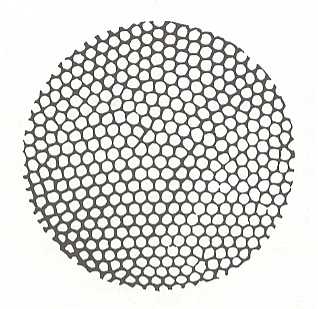
Figure above : Bénard instability. Spatial pattern of convection cells, viewed from above in a liquid heated from below.
(After PRIGOGINE, I. From Being to Becoming, 1980.)
Earlier, namely in the Section "Microscopic consideration of entropy" in Part XXIX Sequel-28 , we introduced Boltzmann's order principle, which relates entropy to probability as expressed by the number of complexions ( = permutations) P. Can we apply this relation here? To each distribution category of (now) the velocities of the molecules corresponds a number of complexions. This number measures the number of ways in which we can realize the velocity distribution category by attributing some velocity to each molecule. As in the case of spatial distributions, the number of complexions of some category of velocity distribution is large when there is disorder -- that is, a wide dispersion of velocities.
[ PRIGOGINE & STENGERS here assume that "the parameters describing crystal structures may be derived from the properties of the molecules of which they are composed, and in particular from the range of their forces of attraction and repulsion", which are "of the order of 10-8 cm, like the distance between the molecules of a crystal".
According to me this reductionist interpretation of the structure of crystals is questionable.
In Part XXIX Sequel-6 we investigated whether such an interpretation is possible, and concluded, as a result of considering branched crystals, that it is probably not, i.e. that branched crystals, such as most snow crystals, show that all crystals whatsoever have holistic features. In one way or another there must be some supramolecular communication between the different parts of a crystal, so that, say, one corner of it 'knows' what the other has done.
In his book "H2O , a biography of water", 1999, BALL, P. writes (p.177/8 of the 2000 Phoenix edition) :
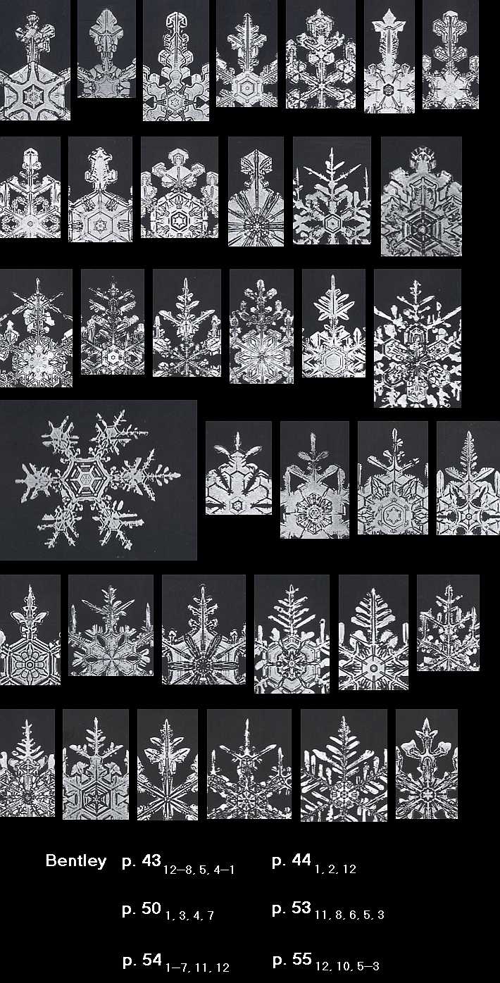
A continuing mystery about dendritic snowflakes is why all six of their branches seem to be more or less identical. The theory of dendritic growth explains why the side branches will develop at certain angles, but it contains no guarantee that they will all appear at equivalent places on different branches, or will grow to the same dimensions. Indeed, these branching events are expected to happen at random. Yet snowflakes can present astonishing examples of coordination, as if each branch knows what the other is doing. One hypothesis is that vibrations of the crystal lattice bounce back and forth through the crystal like standing waves in an organ pipe, providing a degree of coordination and communication in the growth process. Another is that the apparent similarity of the arms is illusory, a result of the spatial constraints imposed because all the branches grow close together at more or less the same rate. But for the present, the secret of the snowflakes endures.That the latter explanation (involving spatial constraints) is incorrect is proven by the two snow crystals that we already depicted earlier in Part XXIX Sequel-4 :
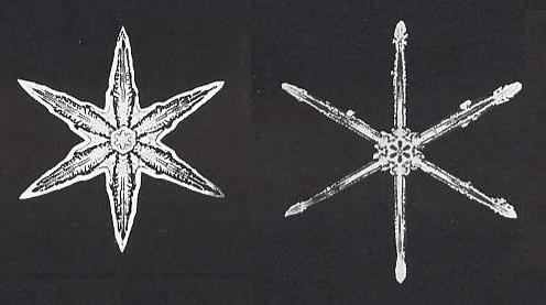
The (main) branches of one and the same crystal are all six of the same morphological type, despite the fact that they have plenty of space to grow in, and do not stand in each other's way. That also the side branches in one and the same crystal are of the same morphological type can be seen in virtually all snow crystals. One (also from Part XXIX Sequel-4) is depicted here :
So crystals (as is indicated by branching phenomena) probably are regulated by global signals or forces. And turning now to branched crystals (dendritic crystals) in particular -- which are probably genuine dissipative structures (far from equilibrium, non-linear) -- we can, at least in a preliminary way, say that they are fully comparable with the structures of the Bénard instability. We will dicuss this further below.
We now return to the discussion of dissipative structures as we found it in PRIGOGINE & STENGERS, Ibid., pp.144. ]
We consider the case of chemical reactions. There are some fundamental differences from the Bénard problem. In the Bénard cell the instability has a simple mechanical origin. When we heat the liquid layer from below, the lower part of the fluid becomes less dense, and the center of gravity rises. It is therefore not surprising that beyond a critical point the system tilts and convection sets in.
But in chemical systems there are no mechanical features of this type. Can we expect any self-organization? Our mental image of chemical reactions corresponds to molecules speeding through space, colliding at random in a chaotic way. Such an image leaves no place for self-organization, and this may be one of the reasons why chemical instabilities have only recently become a subject of interest. There is also another difference. All flows become turbulent (and thus self-organize macroscopically) at a "sufficiently" large distance from equilibrium (the threshold is measured by dimensionless numbers such as Reynold's number). This is not true for chemical reactions. Being far from equilibrium is a necessary requirement but not a sufficient one. For many chemical systems, whatever the constraints imposed and the rate of the chemical changes produced, the stationary state remains stable and arbitrary fluctuations are damped, as is the case in the close-to-equilibrium range. This is true in particular of systems in which we have a chain of transformations of the type A ==> B ==> C ==> D . . . and that may be described by linear differential equations.
The fate of the fluctuations perturbing a chemical system, as well as the kinds of new situations to which it may evolve, thus depend on the detailed mechanism of the chemical reactions. In contrast with close-to-equilibrium situations, the behavior of a far-from-equilibrium system becomes highly specific. There is no longer any universally valid law from which the overall behavior of the system can be deduced. Each system is a separate case. Each set of chemical reactions must be investigated and may well produce a qualitatively different behavior.
Nevertheless, one general result has been obtained, namely a necessary condition for chemical instability : In a chain of chemical reactions occurring in the system, the only reaction stages that, under certain conditions and circumstances, may jeopardize the stability of the stationary state are precisely the "catalytic loops" -- stages in which the product of a chemical reaction is involved in its own synthesis. This is an interesting conclusion, since it brings us closer to some of the fundamental achievements of modern molecular biology.
This concludes our general discussion of far-from-equilibrium systems, following PRIGOGINE & STENGERS in their book Order out of Chaos.
Inorganic far-from-equilbrium chemical systems, and also a model, have been discussed in First Part of Website First Series of Documents : Non-living Dissipative Systems . The reader can consult that document to complete the present discussion about far-from-equilibrium systems.
While in the mentioned document the kinetics and the pattern formation were central, in the next document we will concentrate on the thermodynamics of these far-from-equilibrium systems. For this we will use a more or less simple physical (not chemical) example, namely the Bénard instability, and compare it with the process that leads to branched crystals.
e-mail :
To continue click HERE for further study of the Theory of Layers, Part XXIX Sequel-31.