(Takes a little while loading the images)

e-mail : 

Back to Homepage

We continue with the analysis of the many possible trajectories that -- one for each case, and determined by probabilities -- can emerge from a minimal area in the phase space of the clock doubling system. The minimal area was -- as an example -- set to be the interval 0.0101 of the 0 to 1 line segment.

Now we're going to subject our  unspecifiable number  0.010101----  (which is only specified or defined as to lie in the interval 0.010101) to the clock doubling algorithm (binary point one place to the right, dropping the 1 before the point when it apprears). And we do this as follows :  simultaneously with each round of clock doubling our initial number is extended by one digit (to its right-hand side), the value of which, 0 or 1, is randomly chosen (this we do because our number is supposed to be a number that is, from 0.010101 onwards, unspecifiable, that is to say, undefined). And because at the conclusion of each step in the clock doubling process the number loses one digit at its left side, the lengths of the digit strings that successively appear are equal and remain equal througout the resulting sequence. On the other hand, the initial digit string, representing the system's initial condition, becomes longer and longer, that is to say, the initial number more and more develops, and thus becomes more and more accurately defined and known.
So let's go  ( The digit that is randomly added is indicated in red ) :

Initial number :  0.010101----  ( = First state)
Second state :  0.101011----

(extended) Initial number :  0.0101011----
Third state :  0.010110----

(extended) Initial number :  0.01010110----
Fourth state :  0.101101----

(extended) Initial number :  0.010101101----
Fifth state :  0.011010----

(extended) Initial number :  0.0101011010----
Sixth state :  0.110101----

(extended) Initial number :  0.01010110101----
Seventh state :  0.101010----

(extended) Initial number :  0.010101101010----
Eight state :  0.010100----

(extended) Initial number :  0.0101011010100----
Ninth state :  0.101000----

(extended) Initial number :  0.01010110101000----
Tenth state :  0.010001----

(extended) Initial number :  0.010101101010001----
Eleventh state :  0.100011----

etcetera.

First state :	0.010101----	L
Second state	0.101011----	R
Third state	0.010110----	L
Fourth state	0.101101----	R
Fifth state	0.011010----	L
Sixth state	0.110101----	R
Seventh state	0.101010----	R
Eight state	0.010100----	L
Ninth state	0.101000----	R
Tenth state	0.010001----	L
Eleventh state	0.100011----	R
etcetera.	etcetera.	etc.

Trajectory from 0.010101----  :
0.010101----
0.101011----
0.010110----
0.101101----
0.011010----

Initial number :  0.010110----  ( = First state)
Second state :  0.101100----

(extended) Initial number :  0.0101100----
Third state :  0.011000----

(extended) Initial number :  0.01011000----
Fourth state :  0.110001----

(extended) Initial number :  0.010110001----
Fifth state :  0.100011----

(extended) Initial number :  0.0101100011----
Sixth state :  0.000110----

(extended) Initial number :  0.01011000110----
Seventh state :  0.001101----

(extended) Initial number :  0.010110001101----
Eight state :  0.011010----

(extended) Initial number :  0.0101100011010----
Ninth state :  0.110100----

(extended) Initial number :  0.01011000110100----
Tenth state :  0.101001----

(extended) Initial number :  0.010110001101001----
Eleventh state :  0.010010----

etcetera.

First state :	0.010101----	L	0.010110----	L
Second state	0.101011----	R	0.101100----	R
Third state	0.010110----	L	0.011000----	L
Fourth state	0.101101----	R	0.110001----	R
Fifth state	0.011010----	L	0.100011----	R
Sixth state	0.110101----	R	0.000110----	L
Seventh state	0.101010----	R	0.001101----	L
Eight state	0.010100----	L	0.011010----	L
Ninth state	0.101000----	R	0.110100----	R
Tenth state	0.010001----	L	0.101001----	R
Eleventh state	0.100011----	R	0.010010----	L
etcetera.	etcetera.	etc.	etc.	etc.

Trajectory from 0.010110----  :
0.010110----
0.101100----
0.011000----
0.110001----
0.100011----

So on the basis of all these results we can imagine that from the initial condition 0.0101 (and any other initial condition) many potential trajectories can emanate. Most of them will depart from an unspecifiable number within this initial condition. These trajectories are then, of course, totally erratic and will visit every interval of the 0 to 1 line segment however small, that is to say that in our case the clock doubling system visits every region of its phase space. All the possible trajectories remain within the statistical context formed by the evolution of the whole initial condition (the interval 0.0101).

Randomness is for us, i.e. epistemologically, first of all unpredictability.
It is said that unpredictability is fundamental, i.e. absolute, in the case of a highly unstable dynamical system. This is correct. Whatever refined measuring devises one may invent, such systems remain unpredictable as regards to long-term behavior.
But the assertion that this absolute unpredictability as such implies objective randomness, is not correct by reason of the fact that also in this case the system is unpredictable because  we  are not (and never will be) capable to assess its starting condition with infinite precision (that is required for such systems, that is to say for such highly unstable dynamical systems). And from this exclusively epistemological nature of even absolute unpredictability an objective randomness does not necessarily follow (while it could be present as such). This absolute randomness is only evident when we consider a trajectory of such an unstable system which starts off from (at least) an unspecifiable irrational value, provided such a system can -- in this respect -- be legitimately compared with the (mathematical) clock doubling system. And it is important to know that most numbers are unspecifiable irrational numbers. So our clock doubling system has shown that absolute randomness (as contrasted with randomness which emerges purely by ignorance) is in principle possible. Randomness is thus not inherently epistemological, not necessarily subjective, it can be real, i.e. it can be a real and inherent property of some given dynamical system.
Generally, a trajectory of the clock doubling system, starting off from the volume-like initial condition is erratic, and eventually visits every region of phase space however small this region is taken to be (See the Figure given earlier  :  If we would follow the trajectory still further, we will see that it visits every region of the 0 to 1 line segment, because the digits of the starting number are randomly added, expressing the fact that this number is, apart from its location in a given interval, unspecifiable). In this respect the trajectory is not impeded by its necessary remaining within the bounds of the statistical context or area (brown in the Figure, and determined by the [evolution of the] initial interval), because this statistical context will itself finally cover the whole 0 to 1 line segment (i.e. the whole of the system's phase space). This "eventually visiting every region of phase space" is not because the stastistical context is eventually spreading all over phase space. The spreading of the statistical context or area does not refer to a single trajectory but to the whole of all potential trajectories emanating from the initial volume-like condition, and expresses the eventual loss of all predictability.
When the trajectory is finally allowed to visit every region (one after another) of phase space, the system can be said to be in equilibrium.
Let us determine when this is the case. The initial condition is a small area, defined by some interval, say, 0.0101 ,  as in the previous examples. A trajectory starts off from some sub-interval of this interval. This sub-interval, let it be (as in an earlier example) 0.010101 ,  is the (only) specified part of some irrational number that is unspecifiable beyond this sub-interval and which must be written down as 0.010101---- .  When we now apply clock doubling, the resulting states are partly determined in the first five rounds (iterations). After those rounds the resulting states only consist of digits that were randomly added :

Trajectory from 0.010101----  :
0.010101----
0.101011----
0.010110----
0.101101----
0.011010----
0.110101----
0.101010----
0.010100----
0.101000----
0.010001----
0.100011----
etc.

Everywhere along the trajectory each state is determined by the previous state  ( In an existing digit sequence the binary point is shifted one place to the right and the 1 before the point, when it appears, dropped). And the first few digits (appearing after the binary point) are determined by those already given in the initially given digit string of the starting number. But as soon as the binary point has passed those digits initially present, the chance of a 0 appearing after the binary point is precisely the same as that of a 1 appearing after the binary point (50 percent). This means equal probability for the jumping particle to end up in  L  (left compartment of teh 0 to 1 line segment) or in  R .  And this (as contrasting compartments with states) is perhaps a better criterion for the system's condition of equilibrium.

REMARK :
The clock doubling system, starting from an  i r r a t i o n a l  number, seems (but cannot) (within one Poincaré cycle so to say) to be able to visit some number for the second time. If so, the system enters into a loop, contradicting the irrational starting number. Let us generate a part of a trajectory starting off from an unspecified irrational number, using the same method as in the previous two examples :

0. 0010----
0. 0101----
0. 1011----
0. 0110----
0. 1100----
0. 1001----
0. 0010----
0. 0101----
0. 1010----
0. 0100----
etc.

Here we see some numbers appear for the second time, such as the number 0. 0101---- ,  but the number after its second appearance is different  ( 0. 1010---- different from 0. 1011----). But in fact we can never speak of numbers like 0. 0101----  (or any other such number) as seen to repeat in some sequence, because these numbers are only partially known and remain so.

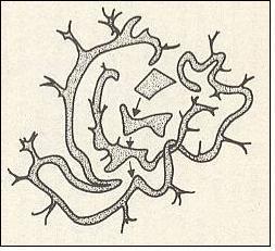
Figure above :  Two-dimensional (in fact 3-dimensional) representation of the evolution of an volume-like initial condition of some unstable dynamical system. The initial area (or volume), representing positive probabilities of system states, eventually is going to extend all over phase space (at least in the sense that it is arbitrarily close to every point of phase space).
This could be interpreted as inevitable relaxation or leveling-out at the statistical level.
(Adapted from COVENEY & HIGHFIELD, The Arrow of Time, 1991)

Figure above :  Diagram of the initial condition as it is represented in the phase space of some dynamical system.
The ontologically smallest area that can represent the initial condition is indicated (red).
The mallest area that represents this initial condition insofar as it can be assessed by observation and measuring -- the epistemological limit -- is indicated (yellow) as being a larger area (containing the ontological limit).

Figure above :  Diagram of the initial condition and of subsequent system states as represented in the phase space of some dynamical system.
The ontologically smallest area that can represent the initial condition and the subsequent system states is indicated (red).
The mallest area that represents this initial condition and the subsequent system states insofar as they can be assessed by observation and measuring -- the epistemological limit -- is indicated (yellow) as being a larger area (containing the ontological limit).
The ontologically statistical context is a still larger area (light blue) -- containing the two smaller areas just considered (epistemological limit and ontological limit) -- indicating the positive probabilities of alternative system states.

Figure above :  Same as previous Figure. Alternative trajectory added.

Figure above :  Same as previous Figure. Alternative trajectory (purple), representing one of the potential trajectories implied by the epistemological uncertainty (yellow) of the initial condition. This trajectory remains within the evolving epistemologically statistical context (greyish area, including the light blue area).
If one assesses after the fact the state the system is in, one finds one out of the many potential small areas (red + yellow) situated in any case within the relevant epistemologically statistical context or area (greyish), while at the same time it could turn out to be situated in the ontologically statistical context or area (light blue) (because this latter context or area is wholly contained within the former).
The system starts from its initial state and then goes through a series of subsequent states. Four of such consecutive states are indicated in phase space and represented not by points but by areas. In fact what they represent is a successive series of points in time. And let us then say that the third one (just choosing one from the sequence) indicates time  t₃  (while the initial condition [initial state] marks time  t₀ ).
The following statements can then be made :

• If somehow we knew not only the initial condition, but also precisely what trajectory actually has emanated from this initial condition, which means that we knew exactly from what point within the red area of the initial condition the trajectory has emanated,  then for time t₃ we can predict, and will indeed find, an area (representing a point, which in turn represents the system's state) at a definite location within the light blue t₃ area (ontologically statistical area). The area indicates the epistemological and ontological uncertainty as to precisely where in phase space the system is, i.e. as to precisely what state the system is in. It is the outcome of an observation or a measurement.

• If we knew the initial condition all the way down to its ontological limit, but no further than that, which means that we knew that the trajectory had started off from one or another point within the red area of the initial condition (while not knowing from precisely which point),  then for time t₃ we can predict only that the system's state will be somewhere in the light blue t₃ area (ontologically statistical area), and indeed will find, after the fact, an area (representing a point [and its uncertainty], which in turn represents the system's state) at a definite location within the light blue t₃ area.

• If we know the intial condition only on the basis of observation and measurements (and this is, of course always the case in scientific practice), that is to say that we (only) know that the trajectory has been started off from one or another point within the yellow area (including the red area) of the initial condition (while not knowing from which point, and even not knowing from which area of that initial condition :  red or yellow [including red] ),  then, for time t₃ we can predict only that the state of the system will be somewhere within the greyish area (including the light blue area), i.e. somewhere within the epistemological statistical context or area. When we measure, after the fact (i.e. at time t₃), we will find an area (representing a point [and its uncertainty], which in turn represents the system's state) indicating the location of the system in this epistemologically statistical area (of phase space).

We will now qualitatively describe the evolution of the initial probability volume (volume-like initial condition) in the phase space of some unstable dynamical system  (It can also be mathematically described, but our mathematical background is not sufficient to do so. Apart from this, I think, that in particular a qualitative description is necessary for the categorical analysis of causality, as we see it at work in unstable dynamical systems. So without taking into account the mathematical description [involving the Liouville equation] I hope that my qualitative description is correct. Maybe some reader finds an error. I would then pleased to hear it from him or her.). The pictorial image which will guide us, is one that we have given already earlier :

Figure above :  Two-dimensional (in fact 3-dimensional) representation of the evolution of an volume-like initial condition of some unstable dynamical system. The initial area (or volume), representing positive probabilities of system states, eventually is going to extend all over phase space (at least in the sense that it comes arbitrarily close to every point of phase space).
This could be interpreted as inevitable relaxation or leveling-out at the statistical level.
(Adapted from COVENEY & HIGHFIELD, The Arrow of Time, 1991)

The initial blob at time  t₀  represents a distribution of positive probabilities of certain very similar and highly ordered configurations (of elements), i.e. the initial configuration of system elements could be this or that highly ordered configuration. Outside this blob are configurations (system states) with zero probability at time t₀ .  When the system starts off, the maximally disordered potential configurations still have zero, or at least very low, probability of being materialized at some little time after t₀ ,  because these maximally disordered potential configurations lie structurally still a long way off from the highly ordered initial configuration. See next Figure.

Figure above :  Two possible configurations of the (16) elements of a dynamical system, representing two states of that system (each represented by a point in phase space). One is highly ordered (image on the left), while the other is highly disordered (image on the right). In order to go from the one to the other the system must go through a number of intermediate states.

In mixing systems (moderately chaotic systems) this end stage can be represented by a very delicate (as compared to the initial blob) structure (see Figure above )  with many tendrils reaching out to every region of phase space. And although its particular shape keeps on changing, its overall shape (i.e. a shape, just such that it reaches into every area of phase space) remains constant, with a very very low probability of the system temporarily falling back to one or another of the more ordered configurations (more ordered states represented by points somewhere in phase space).
What does this final overall shape of the probability distribution function, as it is represented geometrically in phase space (which has, in contrast to our simplified two-dimensional image, many dimensions), namely as the above mentioned delicate structure sending out tendrils to every region of phase space, mean?
Well, while the starting blob only represents a positive probability for a number of highly ordered and similar configurations (states), the end structure (as a morphological type that stays the same) comprises positive probabilities for (almost) every configuration whatsoever, whether ordered or disordered, because now the blob has spread itself all over the phase space of the system, and thus covering (almost) all of the system's potential states. Thus we can say that although at equilibrium each single individual configuration (possible state of the system) has a positive probability for it to materialize (which was not so at the beginning of the system's career), a maximally disordered configuration (that is to say one, or any other of the set of maximally disordered configurations) has (among these positive probabilities) the greatest chance to materialize, simply because there are many more of them. Said differently :  While in the beginning the system can, as regards its next states, explore only a limited area (volume) of phase space, determined by its current statistical context (the currently allowed degree of expansion of the blob), at equilibrium it can explore the whole of phase space, because the statistical context has spread all over it. So the probability distribution function has changed from high probability of one or another ordered configuration (so set at the beginning of the system's career) to high probability of one or another maximally disordered configuration.

Expounded along these qualitative lines it is clear, I hope, that an unstable dynamic system of interacting (and colliding) particles, starting off from some highly ordered state, will, with a very very high probability, evolve to a state of maximum disorder. And, as has been said earlier, because we have argued -- from the assumed fact that point-like initial conditions (and any other point-like system state) not only cannot be determined as such (by us), but also cannot exist -- that the probabilities involved are objective and intrinsic, the ontological status of the particular outcome of the dynamical system is only secondary, while its probabilistic background is primary.

Thermodynamics

Energy

Thermodynamics is about processes mainly from the viewpoint of energy transfer and energy conversion. But what is energy?

Although this definition is supportable only in mechanical terms, it is nevertheless the broadest possible definition.
[ Thermodynamics demonstrates that a given amount of heat cannot be completely converted into work. But this is not supposed to mean that only a part of a given amount of heat is energy. It does not mean that there are two sorts of heat, one convertible into work and the other not. Heat, as such, can be converted into work, and therefore heat is energy.]
There is a variety of types of energy encountered in thermodynamic systems of which we mention potential energy, kinetic energy, heat energy, electrical energy, and chemical energy.
P o t e n t i a l  e n e r g y  refers to the energy that a substance possesses because of its position relative to a second possible position. A stretched spring possesses potential energy and does work as it springs back (i.e. as it is allowed to unstretch). Similarly, water behind a dam possesses potential energy that can be obtained if the water is made to turn a turbine while going through the dam. The energy released by both systems (spring, dam) is transformed into kinetic energy of some object (the spring itself [or other things it draws with it], blades of a turbine) that is moving. Thus the energy possessed by a moving object is called  k i n e t i c  e n e r g y.
C h e m i c a l  e n e r g y  is the potential energy stored in chemical elements or compounds that can be released during a chemical reaction or a physical transformation. The chemical energy stored in elements and compounds determines the reactions that these substances will undergo. And most life processes can be discussed in terms of the storage and release of chemical energy. The chemical energy required or generated may be in the form of either heat or electrical energy. (OUELLETTE, R. Introductory Chemistry, 1970, p.15-16).

The considerations, regarding thermodynamics, that will now follow are largely taken from the textbook of  R.WEIDNER, Physics, 1989, pp. 469, but also from some other sources.

In all the sections that follow, "the system" may consist of any well-defined collection of objects. The system could be a single spring, or a magnet, or some complicated gadget with many internal moving parts. Or the system can simply be an ideal gas (which is, to begin with, a diluted gas) in a container. Actually, we shall use an ideal gas to illustrate thermodynamic processes because the behavior of such an ideal gas is well known. Its equation of state is the general gas law :

Where V = volume, T = temperature, and p = pressure

This law says that V is proportional to the quotient of T and p ( the proportionality constant turns the proportionality relation into an equality relation).

A system is said to be in thermodynamic equilibrium when :

• It is in mechanical equilibrium with the resultant force, and the resultant torque on it is zero.
• It is in chemical equilibrium, and no chemical reactions take place.
• It is in thermal equilibrium, and all its parts as well as its environment are at the same temperature.

• A reversible process can be made to run backward merely by reversing the direction in which the thermodynamic variables change.
• An irreversible process cannot.

No heat enters or leaves the system in this irreversible process (Q = 0), and the gas does no work when it expands freely (W = 0)  [ The gas does not increase its volume by pushing away a piston ].  Therefore, from the First Law,  DELTA (U) = Q - W = 0   [ For work done on the gas this law reads DELTA (U) = Q + W,  while for work done by the gas it reads DELTA (U) = Q - W  ].  Since the temperature is directly proportional to the internal energy for an ideal gas, the free expansion represents an irreversible adiabatic expansion in which the temperature is the same in the final equilibrium state as in the initial state  ( This free expansion can not be described, however, as an isothermal expansion, even though the initial and final temperatures are the same. The expansion proceeds irreversibly. During this expansion, thermal equilibrium does not exist and a temperature cannot be defined for the system  [ When there is no thermal equilibrium, there are temperature differences between its parts or between it and its environment, so at least when its parts have different temperatures there is no definite temperature for the system as a whole ].

The above described free expansion of an ideal gas cannot be represented by a path in a  pV  diagram, but only by its begining and end points.

A reversible process must in general consist of a succession of infinitesimal changes taking place slowly, so that at each stage the system is in thermodynamic equilibrium. Then, and only then, can a temperature be defined for all intermediate stages.

A process is isothermal when during the process the temperature of the system remains the same.
A process is isobaric when during the process the pressure of the system remains the same.
A process is isovolumetric when during the process the volume of the system remains the same.
A process is adiabatic when during the process there is no exchange of heat between the system and its environment. This can be accomplished by thermally insulating the system from its environment.

Any isothermal process is reversible. The temperature remains constant throughout the system, and the system is always in thermal equilibrium as its state changes.
A non-isothermal process, on the other hand, may or may not be reversible. Consider an adiabatic process  ( Here, a temperature change cannot be made undone by exchange of heat with the environment, so this is a non-isothermal process). If a process is to be both adiabatic and reversible, the process must take place fast enough that no thermal energy enters or leaves the system, but slowly enough that the system is at all times in thermal equilibrium. Such conditions can be achieved when the system is inside a good thermal insulator.
There are many examples of irreversible processes :  a bursting balloon, a dropped egg, an overstretched spring, etc.).
A perfectly reversible process is virtually unattainable. In the real macroscopic world, all transformations are somewhat irreversible.
Consider an ideal gas undergoing a reversible process from some initial state  ( p_i ,  V_i ,  T_i )  to some final state  ( p_f ,  V_f ,  T_f ).  According to the First Law of Thermodynamics, the heat  Q_if  supplied to the system, the work W_if done by the system, and the change in the system's internal energy  DELTA (U_if)  in going from  i  to  f  are related by :

Both  Q_if  and  W_if  depend on the process leading from  i  to  f ,  but  DELTA (U_if) = U_f - U_i  does not. The internal energy of an ideal gas is a function of the state of the system, not of its history.
The next three Figures are about three possible reversible paths on  a  pV  diagram (i.e. a pressure-volume diagram) between the same pair of initial and final states. The first two Figures are auxiliary Figures, serving to understand the third Figure, in which the three possible processes are depicted.

Figure above :  Pressure-Volume Diagram depicting two possible states (black dots) of an ideal gas.  The thin curved lines represent isotherms, which means that along such a line the temperature remains constant. There are two such isotherms, one representing a higher temperature, and one a lower temperature.

Figure above :  Same as previous Figure. Initial pressure, final pressure, initial volume, and final volume indicated.

Figure above :  Three reversible paths leading from state  i  to state  f  at a lower temperature.
(a)  Isobaric expansion followed by isovolumetric cooling.
(b)  Isothermal expansion followed by adiabatic expansion.
(c)  Adiabatic expansion followed by isothermal expansion.

• The gas expands at first isobarically and then isovolumetrically.
• The gas expands at first isothermally and then adiabatically.
• The gas expands at first adiabatically and then isothermally.

( First Law of Thermodynamics. If the work was done on the gas (instead of delivered by it), then this Law reads :  Q_if = DELTA (U_if) - W_if  )

DELTA (U_if) is negative, so  minus DELTA (U_if)  is positive, consequently we have :

The three processes shown above are reversible. Indeed, a process can be represented by a continuous line on  a  pV  diagram only if it is reversible. Only then does the system progress through a succession of states of thermal equilibrium with a well-defined temperature at each stage.
For an irreversible process, one can show the two end points (i.e. the initial and final point) on  a  pV  diagram, but no continuous line can be drawn connecting them.
Now suppose that the three above processes are exactly reversed. The system now undergoes compression, rather than expansion. From state  f  to  i ,  the internal energy change is now positive, heat is removed from the system, and work is done on it (volume gets smaller). Whenever a system undergoes a reversible process in which heat is converted to work, one may rerun the process to return the system to its initial state, with work then being converted to heat. The overall change in the internal energy over this special cycle is then zero. Moreover, since the overall process is represented by a single closed line (i.e. the system can go to and fro over that same line) on  a  pV  diagram, rather than a loop, the heat entering the system over the entire cycle is zero, and the work done by the system over the entire cycle is also zero.

U = internal energy of the system.
U_i = internal energy of system in initial state.
U_f = internal energy of system in final state.
U₁ = internal energy of system in state 1.
U₂ = internal energy of system in state 2.
T = (absolute) temperature.
W = work.
W_on = work done on the system.
W_by = work delivered by the system.
V = volume.
p = pressure.
Q = transported heat.
Q_h = heat supplied to the system (heat taken in by the system).
Q_c = heat removed from the system (heat leaving the system).
dX = (infinitesimally) small increase or decrease of quantity X.
=  summation of small quantities (say, dX) over the process-path (leading) from
          state 1 to state 2 of the system.
>  =  larger than.
<  =  smaller than.

The quantities  W_on  and  W_by  already carry their sign, indicated by "on" and "by".

In the following text we do not distinguish between complete and partial differentials (among U, W and Q, only a small increase of U, that is to say dU, can represent a complete differential). All of these small quantities are indicated by  d  (as  in  dX ).

If we add to a system, for instance a cylinder filled with gas below a piston, a small amount of heat  dQ ,  and at the same time perform a small amount of work  dW_on  on the gas, for instance by compressing it, then, as a result, the internal energy U of the system must have increased by

If the amounts of Q and W are large, we must add all the successive small increases by integration. For U this is not necessary (we can just add up all the  dU's ).
So if the change of the system is not small, for example because we add much heat, and compress the gas strongly, then we get :

where 2 and 1 are respectively the final state and initial state, and where the sum of the small changes in (internal) energy is

that is to say the energy difference between final and initial state.
This (i.e. equation (1)) is called the First Law of Thermodynamics, which formulates the law of energy conservation in the theory of heat.
From  dU = dQ + dW_on  (First Law) we have  dW_on = dU - dQ,  and from this in turn we have  dW_by = dQ - dU, which means that a system delivers work only when energy is transported into it. So the First Law says that work delivered by any system is not for free. A machine that could do this is called a perpetuum mobile of the 1st kind.

As a special case, for a process in which no heat is transferred (dQ = 0) into or out of the system, a so-called  adiabatic process ,  the total work done on the system (and the process being an adiabatic compression) is equal to its energy increase :

If we want this adiabatic process to deliver work, i.e. when we have adiabatic expansion, we get :

Work is delivered at the cost of the system's internal energy :
The delivered work is positive, that is to say the left-hand part of the above equation is positive, and so is the whole right-hand part.  U₁ is the initial internal energy of the system and is therefore supposed to be positive. So we can conclude that in absulute values
U₂ < U₁ which means that also here the delivered work is not for free.

The next four Figures illustrate adiabatic and isothermal processes or transformations, still with respect to a gas contained in a cylinder under a piston.

Figure above :  Adiabatic compression (from state 1 to state 2).
Work done on the system is equal to the surface (light blue) under the curve.
Adiabatic compression can be acomplished by pushing a piston (by a force K) in the indicated direction (i.e. from right to left), so that it compresses the gas. No heat can be exchanged with the environment, as indicated by the thermal insulator (yellow).
The applied work can be expressed in several ways :

• By the difference between the internal energies (U) of final state and initial state.
• By the movement of the piston over added distances dx, which causes the volume of the gas to decrease :
  K.dx = p.O.dx = - pdV ,  where O is the surface of the piston, K the force applied to it and dV the change in volume.
  In the first two expressions (terms) the sign (positive or negative) is already being accounted for in the (direction of the) force, that is to say in the direction of dx, but not so in volume and pressure. Therefore the last expression starts with a minus sign, expressing the fact that the work is negative, i.e. done on the system.

Figure above :  Adiabatic expansion (from state 1 to state 2).
Work performed by the system is equal to the surface (light blue) under the curve.
This work consists in the piston being pushed (by the system) to the right :  Initially the gas is in a compressed state, then it expands spontaneously.

Figure above :  Isothermal compression (from state 1 to state 2).
Work done on the system is equal to the surface (light blue) under the curve.
The system is not thermally insulated. Heat Q_c resulting from the compression (piston pushed to the left) is removed from the system, such that the temperature is to remain constant.

Figure above :  Isothermal expansion (from state 1 to state 2).
Work done by the system is equal to the surface (light blue) under the curve.
The system is not thermally insulated. Heat Q_h is taken in by the system, such that the temperature is to remain constant.

This energy is called the heat function for constant volume. See next Figure.

Figure above :  A volume of gas is heated. Because the piston cannot move (it is fixed in position) the volume of the gas remains constant.

Figure above :  A gas is heated. The gas is under a displaceable piston. The weight on top of the piston exercises a force in the downward direction (red arrow). This force causes the gas to have a certain pressure. And because the force is constant, the pressure of the gas is constant. The added heat causes the internal energy of the system to increase and the system to perform work (piston is pushed upward).
If we consider small changes, then we have :
dU = dQ + dW_on  (First Law of Thermodynamics) (Work done on the system).
dU = dQ - dW_by  (Work performed by the system).
dQ = dU + dW_by 
dW = pdV  (change of work is equal to pressure [which is constant] times change of volume)
dQ = dU + pdV
U + pV = H
dU + pdV (pressure constant) = dH  (change of enthalpy)
dQ = dU + pdV = dH  (change of enthalpy).

We have found two heat functions :

• Heat function at constant volume :
  
• Heat function at constant pressure (enthalpy) :
  

If we exert mechanical work on a liquid, for instance by letting blades turn in this liquid, then the liquid gets warmer (Also if we compress a gas adiabatically its temperature increases). But the same end state could have been reached just by heating the liquid (or the gas). So generally, in a series of changes, the end state does not determine the total heat supplied or the total work done on the system.
But the sum of the heat supplied and the work done on the system is determined, it is determined in virtue of the First Law of Thermodynamics (dU = dQ + dW_on), because this sum equals the energy difference between initial and final state.
If we transform a gas with pressure p₁ and temperature T₁ by adiabatically compressing it, into another state with higher pressure p₂ and temperature T₂ ,  then we must apply more work than when we first isothermally compress and then heat the system at constant volume. See next Figure.

Figure above :  The heat supplied to the system depends on the way, along which, from the initial state 1, the final state 2 is reached.

If the change of state is not small, then for a process holds that the sum of the added reduced heats  is equal to the increase of entropy of the system :

This is the  Second Law of Thermodynamics  for reversible systems, i.e. the condition for this law (thus when it has an equality sign) to hold is :  all intermediate stages of the process that are passed through by it must be equilibrium states, the process must be a reversible process. This will generally be the case where the processes are slow.
On the other hand, if this condition is not met, then the added reduced heat is smaller than the entropy increase

and so also (taking all the  dQ / T 's  together) :

This is the  Second Law of Thermodynamics  for irreversible systems.
So (more) generally the Second Law of Thermodynamics (in one of its many equivalent formulations) reads :

In words :  The total of added reduced heats in any process, whether reversible or irreversible, is equal to, or smaller than, the entropy increase of the system.

Just another thermodynamic potential is the free energy.
In the case of an isothermal process, in which the heat  dQ  is always added at the same temperature T, the sum of the added heats is, according to the Second Law, equal to
TS₂ - TS₁ . Let's see how :

Because any isothermal process is reversible, we have :

  (Second Law for reversible systems)

If we multiply both sides of this equation by  T  we get

We now introduce a new function (a new thermodynamic potential), the so-called  free energy  F = U - TS, which also (because U, T and S are) is a function of the state of the given system.
So the work done on the system in an isothermal process, can be determined as follows :

This is equivalent to

And because

we get

In words :  The work done on the system is equal to the increase of free energy.

When the system performs work, then this work is equal to the decrease of free energy :

So in isothermal processes this free energy plays the role of the energy U in adiabatic processes, where we have :

For example an ideal gas that is compressed in a cylinder at a temperature equal to that of the surroundings, possesses an energy which is equal to that of the expanded gas at the same temperature  ( The internal energy of an ideal gas does not change in an isothermal process [WEIDNER, Physics, 1989, p.479] ),  but it has a higher free energy. And indeed we can let the compressed gas perform work by letting it expand isothermally, whereby it takes in heat from the environment (ENSIE, IV, 1949, p.186).
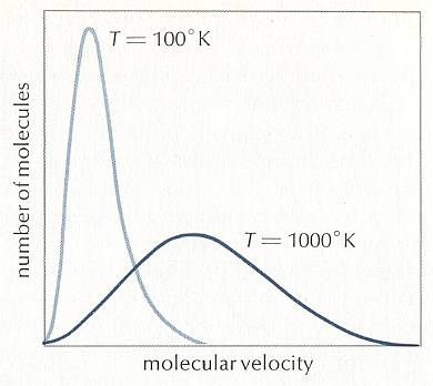
Qualitatively this might be (roughly) explained as follows :
On isothermal expansion of a gas, the temperature T remains constant, and this means that the average kinetic energy of the gas molecules (or atoms) remains the same after the expansion. Because we here are considering an ideal gas, we can disregard the interactions between the molecules, meaning that the energy of the gas is completely represented by this kinetic energy of the molecules. Not all of this energy of the gas, when it is in its (mildly) compressed state, is free energy (which as such is energy that can be converted into work). Only a part of the total energy of the compressed gas is free energy. On isothermal expansion heat is imported from the surroundings. And this heat compensates for (but is itself not totally converted into work) the loss of energy effected by the work done by the gas, i.e. it compensates for the loss of free energy.
We can elaborate on  free energy  a little more.
When an isolated system, like a gas in a well-insulated container, is in its most random state, it has achieved thermodynamic equilibrium. Then a single quantity, the maximum possible value of the entropy, is all that is needed to describe the macroscopic state of equilibrium and the end point of dynamic evolution. But for closed (possible exchange of energy with the environment, but no exchange of matter, for instance a bottle filled with gas or liquid) and open systems (both energy and material exchange is possible, for example an organism), which have an increasingly important dialogue with their surroundings, the state of maximum entropy must take into acount the entropy of the surroundings as well.
If a crystal is melting (which is an isothermal process) heat energy is taken up from the environment, and this heat energy does not increase the temperature. Instead it is used to increase the kinetic energy of the molecules, resulting in the fact that the crystal structure will be disrupted. If, on the other hand, a crystal is forming from a melt (which is also an isothermal process) this heat energy is exhausted to the environment again (where the entropy then increases). This is a nuisance if we wish to investigate the equilibrium properties of the crystal alone. For the sake of simplicity, we wish to avoid bringing the behavior of the environment explicitly into the discussion.
To exclude this environment, we can call on a new quantity, called free energy (as defined above), which assumes its minimum value at equilibrium. The free energy of a system represents the maximum amount of useful work obtainable from it. Although free energy is only a disguised form of the total entropy, its value is that it can be thought of as an intrinsic property of the crystal, thus removing the need to refer to what is happening in the environment. Free energy plays a central role throughout physics and chemistry in describing the equilibrium properties of systems, whether they be magnetic materials, refrigerators or chemically reacting mixtures.
Entropy and free energy are examples of thermodynamic potentials. By this we mean that their respective extrema -- the highest value of entropy and the lowest value of free energy -- reveal the position of thermodynamic equilibrium.
The extrema of thermodynamic potentials act as attractors for the system's evolution through time (COVENY & HIGHFIELD, The Arrow of Time, 1991).
As has been said, the free energy F is equal to U - TS, where U is the energy of the system and T is the temperature (measured on the Kelvin scale). This formula signifies that equilibrium is the result of competition between energy and entropy. Temperature is what determines the relative weight of the two factors.
At low temperatures, energy prevails (which means that it is predominantly energy that must go to a minimum), and we have the formation of ordered (weak-entropy) and low-energy structures such as crystals. Inside these structures each molecule interacts with its neighbors, and the kinetic energy involved is small compared with the potential energy that results from the interactions of each molecule with its neighbors. We can imagine each particle as imprisoned by its interactions with its neighbors.
At high temperatures, however, entropy is dominant and so is molecular disorder. The importance of relative motion increases, and the regularity of the crystal is disrupted. As the temperature increases, we first have the liquid state, then the gaseous state. As has been said, the extremes of thermodynamic potentials such as entropy and free energy define the attractor states toward which systems whose boundary conditions (isolated system, open system) correspond to the definition of these potentials tend spontaneously. Boundary conditions that correspond to entropy involve the isolation of the system from its environment, while those that correspond to free energy involve the openess of the system to its environment (PRIGOGINE & STENGERS, Order out of Chaos, Flamingo edition, 1986, p.126).

In addition to the mentioned characteristic functions as entropy, energy, enthalpy and free energy, there is another one, which is called  THE thermodynamic potential  or  free enthalpy  G = U + pV - TS = H - TS  (where H is the enthalpy).

The theory of heat gives the exact methods to calculate at any given state of a system the corresponding entropy. It teaches to compute how much the entropy increases if we raise the temperature at constant volume (isovolumetric heating), and how much it decreases if we decrease volume at a constant temperature (isothermal compression).
In this way the entropy of an ideal gas given by

where log is the natural logarithm, C_v the specific heat at constant volume, T the temperature, V volume and R the gas constant. The additive constant is undetermined and does not have physical consequences (ENSIE, IV, 1949, p.186).
Generally one can say :  the higher the degree of disorder of the motions of the molecules, the higher the entropy. A way of seeing things which receives more of exact content in statistical mechanics. The solid phase (of a substance) at absolute zero temperature, the most ordered state that can be imagined, with stationary molecules or atoms regularly positioned at certain distances from each other, should then have the lowest entropy.

In 1906 Nernst has put forward the hypothesis, often called Nernst's theorem or also Third Law of Thermodynamics,  that the entropy of all phases (solid, liquid, gas) of a given substance should have the same value at absolute zero temperature, which value was, later, by Planck, significantly, set equal to zero. Although experiments at absolute zero itself are not possible, it turns out that when one approaches absolute zero the theorem of Nernst is being increasingly satisfied. Quantum theory can explain this Law.

If we consider an isolated system, to which no heat is supplied (dQ = 0), then it follows from the Second Law, that for every process taking place in this system  S₂ - S₁ is equal to, or larger than, zero, meaning that the entropy can only increase or at most remains constant :

If the Universe can be considered to be an isolated system, for which the Second law applies, then the entropy of the Universe as a whole can only increase (because most processes taking place in this Universe are irreversible), until a state of equilibrium, of maximal entropy, finally is reached (ENSIE, IV, 1949, p.186). But here the possible effects of gravity (which play a paramount role in the Universe as a whole) are not yet considered.
If we express the Second Law as meaning that the entropy always increases or at most remains constant, then it is only valid for isolated systems, whereas this Law expressed as meaning that the sum of the added reduced heats is equal to, or smaller than, the increase of entropy (see the equation given above ), is valid for all systems.

In what follows we will dig deeper into the concept of entropy and into the meaning of the Second Law of Thermodynamics. For this we must accumulate more insight into the Carnot cycle.
Much of the following is taken from WEIDNER, Physics, 1989, pp. 471.

To use the energy stored in chemical or nuclear fuels, such as coal, oil, natural gas, or uranium, one typically first converts the fuel's potential energy to thermal energy and then converts some of the thermal energy to work. Chemical or nuclear potential energy can be converted to thermal energy with 100% efficiency (for example, by oxidation or nuclear fission). We shall see, however, that a process in which heat is converted to work through the use of a heat engine operating over a cycle can never have 100% efficiency.
Before we consider how to achieve the maximum efficiency for a heat engine, we first note some general properties of any heat engine (such as a steam engine) and heat pump (such as a refrigerator).
A heat engine is defined as any device that in operating through a cycle, converts (some) heat to work and discards the remainder into a cold reservoir. A heat engine is always returned to its initial state in a cycle. Most ordinary heat engines contain a gas as the working substance.  The heat engines we consider are idealized, they have no friction.  But even if somehow no energy at all is dissipated in friction, an engine can never be perfectly efficient. The reasons are far more fundamental.
A heat pump is just a heat engine run backward. More specifically, a heat pump is a device that in operating through a cycle, converts work into heat, at the same time transferring heat from a low- to a high-temperature reservoir. A familiar example of a heat pump is, as has been said, an ordinary refrigerator.
The most general type of heat engine is shown schematically in the next Figure. We skip any mechanical details of construction.

Figure above : 
(a)  Generalized form of a heat engine.
(b)  Energy flow for a heat engine operating between the temperatures  T_h  and  T_c  .

Here W is the work out per cycle and  Q_in  is the heat in per cycle. This definition makes sense in that it compares what we get out of the engine in useful work with what we pay for in heat in. Since we suppose that all the heat enters at the same high temperature  T_h ,  we can write  Q_in = Q_h .
Now we're going to apply the First Law of Thermodynamics to one cycle.
The First Law is about energy conservation. It is not merely about engines. It generally says that the change of internal energy of any system is equal to the sum of the change of heat and the work applied to, or perfomed by, the system. If this change of heat consists in heat supplied to the system, and the work consists in work done on the system, then it says that the (resulting) increase of internal energy of that system (for instance a cylinder of gas with a movable piston) is equal to the sum of the supplied heat and the work done on the system (pushing the piston). For very small amounts it reads :  dU = dQ + dW .
If the supply of heat does not take place during a longer time (implying -- if it did -- a successive series of different small increments of heat), but takes place more or less in a single moment, we can write for  dQ :
DELTA (Q)  or simply  Q  (instead of witing it with an integral  ),  which then means the instantaneous supply of heat to the system. The same goes for the work done on the system :  W is the instantaneous work done on the system (for example compressing a gas). The internal energy of the system then instantaneously changes. This change can be written by DELTA (U).
So we can now rewrite the First Law (now referring to more or less instantaneous processes [heat intake, work applied] ) :

and emphasizing that the work W is done on the system :

Returning now to our heat engine, we have to do with work done by the system (here the engine), and then the First Law must be written accordingly :

which is equivalent to

Here Q is the netto heat added (which is what counts in the First Law).
In our heat engine this netto heat is Q_h - Q_c .
So Q = Q_h - Q_c .
And thus we get :

And because we consider one cycle, i.e. starting from initial condition  i ,  and finally returning to that same condition, the netto change of the internal energy is zero, that is to say DELTA (U) = 0.
So we get :

which is of course equivalent to :

This says simply that work out equals net heat in.

Using this result in the formula (equation (2)) of thermal efficiency stated above we obtain :

This relation shows that an engine can have 100 percent thermal efficiency only if Q_c = 0.  An engine can be perfectly efficient only if no thermal energy is exhausted to the cold reservoir. A perfectly efficient heat engine would convert all the thermal energy entering it to work output when operated over a complete cycle, discarding none. This is impossible.
The reason?  The Second Law of Thermodynamics.  Like any other fundamental law in physics, it is confirmed by the circumstances that no exception to it has ever been found.
We shall encounter the second law of thermodynamics in several different but equivalent formulations. We have already encountered the second law as it relates to the behavior of a system of numerous particles, which always proceeds to states of greater disorder.
Our first statement of the second law of thermodynamics is as follows :

No heat engine, reversible or irreversible, operating in a cycle, can take in thermal energy from its surroundings and convert all this thermal energy to work.

That is to say :

Where  Q_h  is the heat supplied to the engine,  Q_c  is the heat handed over to the environment, and W is the work performed by the ideal engine (i.e. an engine with no friction).
For any cyclic engine, Q_c > 0, and  e_th < 100 percent.

Figure above :
(a)  Generalized form of a heat pump.
(b)  Energy flow for a heat pump operating between the temperatures T_h and T_c  .

where Q is the netto heat taken in.
And when emphasizing that the work W is done on the system, we write :

And because we consider one complete cycle (where thus the system has returned to its original state) DELTA (U) = 0  (i.e. no net change in internal energy). So we get :

In the heat pump, heat in the amount of  Q_c  is taken in (from the cold reservoir [see drawing above] ), while eventually more heat (i.e. more heat than was taken in) in the amount of  Q_h  is exhausted (to the hot reservoir). So the  netto  amount of heat taken in is  Q_c - Q_h .  So  Q = Q_c - Q_h  (because Q [as it figures in the First Law as just stated] is the net heat supplied to the system  [ In fact Q is just the supplied heat, but in the context of heat engines or heat pumps we must make a difference between initial heat intake and net heat intake).
And now the above equation is equivalent to :

which in turn is equivalent to :

where  Q_h  is exhausted heat, and  Q_c is heat supplied to the pump.  This formulation looks like, but is not the same, as the formulation given above for the second law.
Nevertheless we recognize this as the Second Law, because when we reverse all inherent signs of the terms, that is to say :
heat in ==> heat out,  heat out ==> heat in,  W_on ==> W_by ,  heat pump ==> heat engine,  we obtain the first formulation (of the second law) :

No heat pump, reversible or irreversible, operating over a cycle, can transfer thermal energy from a low-temperature reservoir to a higher-temperature reservoir without having work done on it.

For any cyclic heat pump, W_in ( = W_on) > 0.
This statement of the second law tells us that if a hot body and a cold body are placed in thermal contact and isolated, it is impossible for the hot body to get hotter while the cold body gets colder (for this work is needed), even though this would not violate energy conservation, or the first law of thermodynamics. The observed fact that when a hot object and a cold object are brought together, they reach a final temperature  between  the initial temperatures is an illustration of the second law. Heat can spontaneously flow only from a hot body to a cold body.

The Carnot cycle

Lazare Carnot, the father of the french engineer Sadi Carnot (the latter :  1796-1832), who had produced an influential description of mechanical engines, concluded that in order to obtain maximum efficiency from a mechanical machine it must be built, and made to function, to reduce to a minimum :  shocks, friction, or discontinuous changes of speed -- in short, all that is caused by the sudden contact of bodies moving at different speeds. In doing so he had merely applied the physics of his time :  only continuous phenomena are conservative. All abrupt changes in motion cause an irreversible loss of the "living force". Similarly, the ideal  heat engine,  instead of having to avoid all contacts between bodies moving at different speeds, will have to avoid all contact between bodies having different temperatures.
The cycle for a good heat engine therefore has to be designed so that no temperature change results from direct heat flow between two bodies at different temperatures. Since such flows have no mechanical effect, they would merely lead to a loss of efficiency.
The ideal cycle is thus a rather tricky device that achieves the paradoxical result of a heat transfer between two sources at different temperatures without any contact between bodies of different temperatures. It is divided into four phases. During each of the two isothermal phases, the system is in contact with one of the two heat sources and is kept at the temperature of this source. When in contact with the hot source, it absorbs heat and expands. When in contact with cold source, it loses heat and contracts. The two isothermal phases are linked up by two phases in which the system is isolated from the sources -- that is, heat no longer enters or leaves the system, but the temperature of the latter changes as a result, respectively, of expansion and compression. The volume continues to change until the system has passed from the temperature of one source to that of the other.
Along these lines Sadi Carnot recognized that of all possible heat engines operating between two temperature extremes, the most efficient was a reversible one that would -- to describe it again -- operate as follows :

• Receive thermal energy isothermally from some hot reservoir maintained at a constant temperature T_h .
• Reject thermal energy isothermally to a cold reservoir maintained at a constant temperature T_c .
• Change temperature in reversible adiabatic processes.

Figure above :  A Carnot cycle, consisting of two reversible adiabatic and two isothermal processes, operating between the temperatures  T_h  and  T_c .  The thin black curved lines are isotherms (meaning that along such a line the temperature does not change).
means temperature increment or decrement.
means heat increment or decrement.
The area (light blue) enclosed by the loop is equal to the work W performed by the cycle.

Figure above :  A Carnot cycle, consisting of two reversible adiabatic and two isothermal processes, operating between the temperatures  T_h  and  T_c .  The thin black curved lines are isotherms.
The area (light blue) enclosed by the loop is equal to the work W performed by the cycle.

The thermal efficiency -- by the way -- of any reversible cycle, including the Carnot cycle, is independent of the working substance [steam, air, or whatever] ). So the ratio  Q_c / Q_h  does not depend on the working substance. Therefore, if the engine operates in a Carnot cycle, the ratio  Q_c / Q_h  can depend only on the temperatures  T_h  and  T_c  at which the heat enters and leaves the system (In the two adiabatic steps there is no heat exchange at all with the environment (Q = 0)).
So we can write :

We could say that this is the definition of a (reversible) Carnot cycle, because it is one when this is the case.

By combining the two expressions, we can write the thermal efficiency of a Carnot cycle in terms of temperatures as

This equation gives the maximum (maximum, because it is about a Carnot cycle) thermal efficiency attainable for  any  engine operating between the temperatures  T_h  and  T_c .  We see that it is 100 percent (e_th = 1) only if the engine exhausts heat to a cold reservoir at, and remaining at, the absolute zero of temperature -- clearly an impossibility. It is important to realize that the impossibility of 100 percent efficiency, as established here, is not because of friction, because we here consider ideal engines, that is engines without friction.
Heat engines typically have very low efficiency. For example, if an engine takes in heat at the high temperature 200⁰ C and exhausts heat at room temperature of 30⁰ C  (T_h = 473 K,  T_c = 303 K), its maximum efficiency is  e_th = 1 - (303/473) = 36%.  In any real engine, friction is present, the processes are not perfectly reversible, and the operating cycle is not a Carnot cycle. Consequently, the actual efficiency is even less.

Now we will show (WEIDNER, Physics, 1989, p.478) that the Carnot cycle is the most efficient of all reversible cycles operating between two fixed temperature extremes.
Consider the cycle shown in the next Figure (left image).

Figure above :
Left image :  A non-Carnot cycle operating between  T_h  and  T_c .
Right image :  The reversible expansion can be approximated closely by a series of adiabatic and isothermal expansions.

where  T_c  and  T_h  are the temperature extremes of the working substance in the engine.

Again we will elaborate on the so important thermodynamic variable, the  entropy  of a system. As will be pointed out further below, the entropy is a quantitative measure of the disorder of the many particles that compose any thermodynamic system.
First we will, starting with the Carnot cycle, reason our way to a definition of entropy (in fact a definition of entropy change), and from there we will, in a next Section, arrive at the formulation of the Second Law of Thermodynamics in terms of entropy.

Earlier we had established the following with respect to the Carnot cycle :
If the engine operates in a Carnot cycle, the ratio  Q_c / Q_h  can depend only on the temperatures  T_h  and  T_c  at which the heat enters and leaves the system (In the two adiabatic steps there is no heat exchange at all with the environment (Q = 0)).
So we can write :

From this relation we can derive another very important relation by a simple mathematical manipulation :

The latter equation means that for a reversible Carnot cycle the ratio of heat to temperature (which ratio is called the reduced heat) is the same for both the isothermal expansion and isothermal compression  ( In the adiabatic steps there is no Q ). Or in otherwords :  The ratio of  heat in  and the temperature at which this heat was taken in (and at which isothermal expansion takes place), is equal to the ratio of  heat out  and the temperature at which this heat was taken out (and at which isothermal compression takes place). Or, also :  In a Carnot cycle the intake of reduced heat  Q / T  is equal (in magnitude) to the exhaust of reduced heat  Q / T.  See next Figure.

In the analysis that follows we adhere to the following sign convention :
Heat entering the system is positive.
Heat leaving the system is negative.
Using this convention, we then have for the Carnot cycle

Figure above :  A reversible cycle approximated by Carnot cycles (light blue, yellow, green).

holds for each of these.  Adding the equations for the individual small Carnot cycles that approximate the original reversible cycle, we have

We see that no heat enters or leaves the system apart from the processes at the perifery :

Q₁ in, Q'₁ out,
Q₂ in, Q'₂ out,
Q₃ in, Q'₃ out.

Therefore, we can write the last equation more generally as

where  Q  stands for the netto heat intake  (Q₁ in + Q'₁ out, etc. [where the signs are already accounted for] )  and  T  stands for the temperatures at which intake or exhaust of heat took place. The summation is taken around the perifery of the original cycle. In the limit (i.e. when we have taken the smallest possible junior Carnot cycles, in order to obtain a most accurate approximation), we can then write

The circle on the integral sign indicates that the integration is to be taken around a closed path. We can call this integral  a  loop integral.
In words the last expression says that for any reversible cycle, the sum of the quantities giving the ratio  dQ / T  of the heat  dQ  entering the system to the temperature  T  at which the heat enters  is  zero around the cycle.
This is equivalent to saying that the integral (i.e. now the path integral) of  dQ / T  between any initial state  i  and any final state  f  is the same for all reversible paths from  i  to  f .  Let's explain this :

If we add up the two paths of the above Figure (paths, both starting from  i  and both ending up at  f )  while, with our adding, starting at  i ,  and going around the whole loop, and thus ending up at  i  again, we get, when we take the inherent directions of the two paths into account :

P₁ + (-P₂)  [ = going around the whole loop] = 0
This is equivalent to
P₁ - P₂ = 0
which is equivant to
P₁ = P₂

So along the path  P₁  equals along the path  P₂  between the same end points  i  and  f .

We will now proceed further to arrive at a (macroscopic) definition of entropy (change) by using an anlogy :  With a reversible cycle (a Carnot cycle or a non-Carnot cycle) we have to do with a process course going from some starting point and finally ending up at this same starting point again, and where the summation of some quantity is equal to zero. Precisely the same is the case of a conservative force. And this gives us an idea of how to define entropy (macroscopically).
So we exploit a mathematical property that obtains in the relation between a conservative force  F  (which is a vector) and the associated potential energy  U  of the system  [ For example, the wind is a conservative force (field) :  If we, when taking a ride, experience fair wind, we 'pay' for that in terms of unfair wind when we return (along whatever path) back to where we started from ].  The potential energy difference between two end points  i  and  f  is related to the conservative force by

where F (force) and  r  (way in the direction of the force) are vectors. If  U_f  is smaller than  U_i ,  then we have a force. In the formula  U_f  is considered larger than  U_i ,  so there must be a minus sign before the integral.
This relation can be written, however, only if the force is conservative and

with the net work (force x way) done by the conservative force equal to zero over a closed loop.

In like fashion we may  define  a thermodynamic quantity, called the  entropy S, whose difference depends only on the end points. By definition (indicated by  ),

Note that the integration may be carried out along  any reversible  path leading from  i  to  f .  This equation reduces to

(which was established above) when  i = f  around a closed loop.

Now suppose that some system proceeeds irreversibly from state  i  to  f .  We cannot represent any irreversible process by a path on a  pV  diagram. Nevertheless, we can determine the entopy difference between the states  i  and  f .  We simply imagine the system to pass from  i  to  f  along a reversible path connecting the two end points and compute the change in entropy, using the above formula defining entropy difference .  This is allowed because the entropy difference depends only on the end points (as established above, when discussing different paths between the same end points), not on the path (Analogously, in mechanics we can evaluate the potential-energy difference between two points, even when a nonconservative dissipative force also acts and the system is not able to pass reversibly between the end points. We do this by computing the work done by the conservative force alone).
In general, when a system is taken round a complete reversible cycle and returned to its initial state  i ,  the following changes occur. The net change in internal energy is zero  ( DELTA ( U ) = 0 ).  The net change in entropy is zero  ( DELTA (S) = 0 ).  The work W done by the system is equal to the area enclosed by the loop on the  pV  diagram. By the First Law of Thermodynamics, the net heat Q entering the system is then Q = W .
[ In the case of a cycle, as we see it in a heat engine, we must speak of  net  heat entering the system, because we can suppose that there is also heat leaving the system, which means that the total heat entering the system is greater still. The first law is indeed about an energy balance ]  :

DELTA( U ) = Q - W_by  (first law).
DELTA( U ) = 0
0 = Q - W_by
Q = W_by

Now suppose that a system is taken through an irreversible cycle and returned to its initial state  i .  The change in internal energy again is zero  ( DELTA( U ) = 0 ).  The change in entropy is also zero  ( DELTA(S) = 0 ).  The system has done work in the amount W, but it is not representable by any area on a  pV  diagram. Once again, net heat entering the system is Q = W.

Entropy and the Second Law of Thermodynamics

Having obtained a definition of entropy (change), we can now state the Second Law of Thermodynamics in terms of entropy :

For an isolated system the total entropy remains constant in time if all processes occurring within the system are reversible. On the other hand, the total entropy of an isolated system increases with time if any process within the system is irreversible. Since all actual macroscopic systems undergo irreversible processes, the  total entropy of any real system always increases with time.
It is easy to show the equivalence between this statement of the Second Law and the one given earlier, based on heat engine behavior, which read :  The heat  Q_h  supplied to the engine is equal to the sum of heat  Q_c  given off to the environment and work  W_by  done by the engine, meaning that not all heat supplied to the engine can be converted to work :

Q_h = Q_c + W_by

Consider a system composed of a hot reservoir at temperature  T_h ,  a cold reservoir at temperature  T_c ,  and a heat engine operating between the two heat reservoirs, as shown in the next Figure.

Figure above :  The system, consisting of the heat engine together with the hot and cold reservoirs, chosen in applying the second law of thermodynamics to heat engines and in computing entropy changes.

• The hot reservoir loses entropy because heat  Q_h  leaves the reservoir :
  DELTA(S) (hot reservoir) = - Q_h / T_h  (supplied reduced heat to the engine).
• The cold reservoir gains entropy because heat  Q_c  enters the reservoir :
  DELTA(S) (cold reservoir) = Q_c / T_c  (exhausted reduced heat from the engine).
• The heat engine alone undergoes no change in entropy since it is returned to its initial state with the same entropy after completing a cycle, whether the engine is reversible or not.
• Work is done by the engine, and energy leaves the system. But no entropy leaves or enters the system since ordered energy associated with work has no entropy content.

The change in entropy (net gain of entropy) is thus equal to the net reduced heat that is exhausted (to the environment, which here is :  the cold reservoir).
Now recall the definition of the thermal efficiency of any heat engine :

Earlier we proved that no engine operating between the two fixed temperatures  T_h  and  T_c  could be more efficient than a reversible Carnot engine, whose efficiency is

Therefore,

or rewritten (see below ),

That is to say, the exhausted reduced heat is equal to, or greater than, the imported reduced heat. So the first equation obtained above

then gives

which is what we set out to prove, namely the equivalence of the formulation of the Second Law in terms of the features of a heat engine : supplied heat, exhausted heat and work done  and  its formulation in terms of entropy change.

The rewriting done above, can be explained as follows:

We had the inequality (equal to, or smaller than)

Subtracting  1  from both members of this inequality yields the equivalent inequality

From this inequality (equal to, or smaller than) we get an equivalent inverse one (equal to, or greater than) by reversing the inequality sign and changing the minus sign into a plus sign :

The above Figure shows that if we change the signs of both members of an inequality, we get an equivalent relation if we also reverse the inequality sign, so we get

If we turn the quotients upside down, then, in order to obtain an equivalent relation, we must inverse the inequality sign. The following drawing makes this clear.

So we get

Dividing both members by  T_h  gives the equivalent relation

Multiplying both members by  Q_c  gives the equivalent relation

which, of course is equivalent to

Which is indeed the result of the above rewriting .

Earlier we defined  thermodynamic equilibrium  in terms of mechanical, chemical and thermal equilibrium. In thermodynamic systems we can concentrate on the latter.
Thermal equilibrium means that all the parts of the system have the same temperature. Only then can a temperature of the system as a whole be defined. So a system can be at equilibrium while having a temperature  T₁ .  But it can also -- say, later -- be in equilibrium while having a higher (or lower for that matter) temperature  T₂ .  When the process is not too fast, the system can go from a  T₁  equilibrium state to a  T₂  equilibrium state.  So the system can be in equilibrium even if its temperature changes, provided it goes slowly.
In the case of an engine operating as a reversible Carnot cycle, we can say that all four processes (isothermal expansion, adiabatic expansion, isothermal compression, adiabatic compression) can be represented as lines in a  pV  diagram. So the system passes through a long succession of equilibrium states (and only equilibrium states) when it goes through one cycle. The 'motor' that makes this cycling through equilibrium states possible is the temperature difference between the hot reservoir and the cold reservoir which take care for intake and exhaust of energy into and from the engine.
When we heat a layer of liquid from below, a temperature gradient will be set up in the liquid. And as long as this gradient exists the liquid in not in (thermodynamic) equilibrium. By intensifying the heating (from below) the liquid will be pushed further and further away from equilibrium. Finally when the liquid is no longer capable of transporting the heat from bottom to top by conduction alone, its molecules spontaneously organize such that now the heat can be transported by convection, in which the molecules move over macroscopic distances (Such systems, being pushed far away from equilibrium, and then reaching some critical point after which they self-organize, will be discussed in a later document that is about far-from-equilibrium thermodynamics. The processes involved in far-from-equilibrium situations occur in organisms, but also in the generation of dendritic crystals [as seen in snow] ), adding another element to the crystal analogy.
But in a Carnot cycle the system passes through equilibrium states only, which differ from each other with respect to pressure, volume and temperature. But in every single moment the parts of the system have equal temperatures, that is to say the system is in equilibrium.

Microscopic consideration of entropy

Macroscopically entropy is stated in terms of heat and temperature (both are macroscopic variables). The microscopic consideration states entropy in terms of disorder.
To characterize the concept of temperature it was sufficient to involve the average energy of the molecule.  Entropy is about the way by which this energy is distributed among the particles :  The entropy S indicates the degree of randomness.  More precisely :

in which ln is the natural logarithm.  P is the number of ways by which a configuration can result by interchanging the roles of the different particles (permutation), or, equivalently, P is the probability (in terms of the number of permutations) that the system will be in the state it is actually in, compared with all other possible states.   k  is the Boltzmann constant.
So for the most improbable configuration (for instance one particular (i.e. chosen) particle having all the energy of the system, while all the other particles have zero energy) we have  S = 0  (because P = 1, which means that there is only one way to formally accomplish this configuration (all energy must go to that chosen particle. And because log 1 = 0, we get S = 0 ).
If we speak of the probability of a state, we must realize that for every state there is only one way to achieve it, not in the physical sense, but formally, in the sense of a pattern of distribution of velocities or positions among the particles. So when we say that a disordered state is more probable than an ordered one we must not consider particular individual states but categories (configuration categories) of states. Now it is the case that when we describe a given state only as belonging to the category of disordered states, while not distinguishing between the different states that belong to this category, the probability of the system to be in one of these states is greater than it to be in one of the states belonging to the category of ordered states, because there are many more ways (permutations) to formally achieve one of the disordered states than there are ways (permutations) to formally achieve one of the ordered states.
The following explanation of the microscopic definition of entropy is partly taken from R. ADAIR, The Great Design, PARTICLES, FIELDS, and CREATION, 1987, pp.142.
Let us imagine a billiard table (with no side holes) and three colored balls. We further imagine that there is no friction whatsoever when the balls roll over the table and collide. Say that we have a green, black and red ball. Further we have divided the table into three equal areas, which we call 'upper', 'middle', and 'lower' area. We set the three balls in motion by importing energy to the system (say by banging the underside of the table). The balls will then roll around indefinitely because no energy is lost by friction. We then take a set of pictures of the table and balls at random times and classify the pictures as to the configurations of the balls with respect to the three areas. So we consider the distribution of the balls among the three areas (not considering pictures where balls lie on the border between two areas), and do not consider where in such an area a ball lies. We only take into account in what area (upper, middle, lower) a ball of a certain color (green, black, red) lies at the moment a picture was taken.
Because we have three balls, three colors, and three areas, there are 3 x 3 x 3 = 27 possible configurations of the three ball distributed among the three areas. These configurations let themselves be classified into 10 (configurational) categories :

• Category 1 :  In each area one ball.
• Category 2 :  One ball in upper area, two balls in middle area.
• Category 3 :  One ball in upper area, two balls in lower area.
• Category 4 :  Two balls in upper area, one ball in middle area.
• Category 5 :  One ball in middle area, two balls in lower area.
• Category 6 :  Two balls in upper area, one ball in lower area.
• Category 7 :  Two balls in middle area, one ball in lower area.
• Category 8 :  Three balls in upper area.
• Category 9 :  Three balls in middle area.
• Category 10 :  Three balls in lower area.

Figure above :  The ten configurational categories with respect to three balls and three areas (by not accounting for colors we go from individual configurations to categories of configuration).

The First Category consists of six individual configurations, which means that a configuration specified only as to belong to Category 1 can be formally made in six ways :

Figure above :  The six ways to formally construct a configuration specified only as to belong to Category 1.

The Second Category consists of three individual configurations, which means that a configuration specified only as to belong to Category 2 can be formally made in three ways :

Figure above :  The three ways to formally construct a configuration specified only as to belong to Category 2.

The Third Category consists of three individual configurations, which means that a configuration specified only as to belong to Category 3 can be formally made in three ways :

Figure above :  The three ways to formally construct a configuration specified only as to belong to Category 3.

The Fourth Category consists of three individual configurations, which means that a configuration specified only as to belong to Category 4 can be formally made in three ways :

Figure above :  The three ways to formally construct a configuration specified only as to belong to Category 4.

The Fifth Category consists of three individual configurations, which means that a configuration specified only as to belong to Category 5 can be formally made in three ways :

Figure above :  The three ways to formally construct a configuration specified only as to belong to Category 5.

The Sixth Category consists of three individual configurations, which means that a configuration specified only as to belong to Category 6 can be formally made in three ways :

Figure above :  The three ways to formally construct a configuration specified only as to belong to Category 6.

The Seventh Category consists of three individual configurations, which means that a configuration specified only as to belong to Category 7 can be formally made in three ways :

Figure above :  The three ways to formally construct a configuration specified only as to belong to Category 7.

The Eighth Category consists of only one individual configuration, which means that a configuration specified only as to belong to Category 8 can be formally made in one way only :

Figure above :  The one way to formally construct a configuration specified only as to belong to Category 8.

The Ninth Category consists of only one individual configuration, which means that a configuration specified only as to belong to Category 9 can be formally made in one way only :

Figure above :  The one way to formally construct a configuration specified only as to belong to Category 9.

The Tenth Category, finally, consists of only one individual configuration, which means that a configuration specified only as to belong to Category 10 can be formally made in one way only :

Figure above :  The one way to formally construct a configuration specified only as to belong to Category 10.

which is one of the three configurations of  Category 7 ,  we look at the probability that one or another configuration of some given Category (spatially) represents the state of the system at some chosen moment. So we attach a probability to a given Category instead of to a given individual configuration. And because at equilibrium each individual configuration (of which there are 27) has an equal probability to represent the (spatial) state of the system at any one time, a Category has a higher probability to represent the (spatial) state of the system at some chosen time if it contains more individual configurations.
For example  Category 7  consists of three individual configurations (each one of them satisfying the category definition  "two in middle, one in lower" ).  As has been said, each individual configuration (of whatever Category) has a probability of  1 / 27  to represent the state of the system. So if we want to assess the probability of the Category (that is to say of Category 7 ),  we just add up the probabilities of its three constituent configurations :
1 / 27 + 1 / 27 + 1 / 27 = 3 / 27
So the probability that any one of the three configurations (it doesn't matter which one) of Category 7 represents the (spatial) state of the system at some randomly chosen moment  is  3 / 27.
In the same way we find that the probability that any one of the six configurations (it doesn't matter which one) of  Category 1  represents the (spatial) state of the system at some randomly chosen moment  is  6 / 27.
So the probabilities associated with the 10 configurational categories are as follows :

Figure above :  The ten configurational categories (three balls, three areas) and their probabilities
6/27,  3/27,  3/27,  3/27,  3/27,  3/27,  3/27,  1/27,  1/27,  1/27
(which series forms the probability distribution over the ten configurational categories when the system is in equilibrium).

with all three balls in the lower area.
And also, about  1 / 27  of the pictures will show them in the configuration

with all three balls in the middle area,
whereas a much larger proportion, about  6 / 27  of the pictures, will show them in the configuration

with one ball in each area (no matter what color is in what area).
And it is important to note that the proportion of pictures showing, say, the configuration

Now, if we begin with the balls in the highly ordered and unusual configuration

(unusual configuration, because the probability for this configuration [representing Category 10 consisting of only one individual configuration] is only  1 / 27 ),  the balls will tend to go spontaneously to the more disordered pattern

that is to say to one (no matter which) of the six individual configurations of Category 1, because the probability of attaining such a configuration is higher (6/27) than that of the previous configuration (1/27),  whereas if we start with this (category of) disordered configuration, i.e. if we start with one of the individual configurations of Category 1 (one ball in each area), there will be a much smaller chance that the system will spontaneously go to the ordered pattern

Indeed, the probability of going from  order to disorder -- in our case from

The spontaneous reversal of the order-to-disorder change is improbable.

When we consider systems that are more complicated than the simple system of three balls rolling around on a table divided into three parts, the ratio's of probabilities and improbabilities become much greater. If we had divided the table into 10 parts and used 10 balls, for example, the probability of going from an ordered pattern (such that all the balls were in one sector) to a disordered pattern (such that one ball were in each sector) is about 3.6 . 10⁶ times as great as the reverse change from the disordered configuration to the ordered. But this model of 10 balls in 10 places on a pool table is still very, very simple compared to a world of enormous numbers of microscopic molecules and atoms moving in a three-dimensional manifold. Then the improbabilities we found for our simple systems become virtual impossibilities for analogous actions in the real, complex systems found in nature.
It is most important (ADAIR, p.144) to notice that our construction of the relative probabilities (i.e. the  x  of  x / 27  in our example) of the various configurations of balls on the table is largely independent of any consideration of the detailed character of the interactions of the balls with each other or with the sides of the table. In general, the important statistical conclusions or statistical laws we develop are almost independent of the details of individual interactions. Of course, this is why the laws are so general and so powerful.
Summarizing :  With respect to positions we have found that

When the system is in equilibrium, the probability of its state being represented by a spatial configuration of its elements, say balls or particles, (a configuration) that belongs to a certain general  t y p e  (category) of configuration, i.e. a configuration of balls  j u s t  satisfying the definition of that type (category) of configuration (and thus without any other specification being demanded to mention),  depends on the number of ways a configuration satisfying this type can be formally constructed. The more ways there are, the higher the probability, as compared to types with fewer ways to formally construct configurations satisfying them  ( The more cards of a certain type are present in a shuffled deck, the higher the chance that we pick such a card). Of course each configuration belonging to one and the same type has the same probability (of representing the system' state spatially).
The configurational types are here supposed to refer, as types, to degrees of order and disorder. And it is now clear, that configurations, insofar as they belong to types of (spatial)  d i s o r d e r,  are more probable (to represent the system's spatial state) than configurations, insofar as they belong to types of (spatial)  o r d e r.
Generalized, we here have -- in the form of relative statistical probabilities -- the basis for defining  entropy  microscopically, that is in terms of order and disorder of the collection of elements of the system.

For expositional simplicity we have considered only the distribution of the positions of the balls. The momenta (involving mass and velocity) of the balls play a similar role in analyses of probability. As the balls move about the frictionless table and occasionally collide, the momenta of the balls will interchange and there will be a probability distribution of such momenta. For any particular ball -- say, the red ball -- we could measure the momentum of the ball at many random times. The ball would be almost stationary, and have almost no momentum, in very few measurements. Similarly, few measurements would show the red ball with nearly the maximum possible momentum (when the black ball and the green ball were almost stationary), and the red ball had most of the energy of the system). Most of the measurements would show the red ball with a momentum such that the energy of the ball would be about one-third of the total ball-energy. Moreover, a ball with very high or very low energy will tend to come to a state of average energy in time, whereas the reverse change will be improbable :  a ball with an average energy or momentum is not likely to lose all its energy or take up all the energy of the balls on the table. The ball will tend to go from an unlikely momentum (very high, or very low) to a likely momentum.
Just like an enlargement of the table would serve to increase the range of positions that the balls might have, thus increasing the number of ways the balls would be distributed,  an increase in the total energy of the balls, allowing a wider spread of momenta, would increase the number of possible momentum configurations and thus the range of probability.

To make use of the principles presented here that lead to the concept that order goes spontaneously to disorder and not the reverse, we need to define what we mean by order and disorder in a quantitative way.
We then define the quantity entropy in terms of the relative statistical probability  P  of a system's state by equating a change in the entropy with a proportional change in the number of ways the system (that is a state of it) can be formed. With the  relative statistical probability  we mean just the number of ways to form a state category or type (as was the  x  in  x / 27  of the above example, and where  x / 27  was the absolute probability).
But to be able to do this we must first give Boltzmann's microscopic characterization of (just) entropy (S) (without deriving it), and then derive from it the equation for entropy change :

where  P  is the number of ways a state (defined as type) of the system can be formally made, or, equivalently, the number of permutations a given type of state has.
ln  is the natural logarithm, and  k  is the Boltzmann constant, that is the proportionality constant between S  and  ln P.

Boltzmann's constant  k  is the ratio of a characteristic energy of a single particle  to  the temperature of the medium holding the particle. For example, the kinetic energy of a molecule of a gas at an absolute temperature T is :  ( 3/2 )kT, which means that   k = (kinetic energy ( 2/3 )) / T   (ADAIR, p.148, note 1).
An equivalent definition -- given in WEIDNER, 1989, Physics, p.486 -- reads :   k = R / N_A ,   where  N_A  is Avogadro's number (i.e. the number of particles [atoms, molecules] in a mole of the gas [where  a  mole  is the number of grams of the gas equal in magnitude to the relative molecular mass of the gas],  and  R  is the universal gas constant  figuring in the general gas law :   pV = nRT   ( p = pressure, V = volume, T = absolute temperature,  n = number of moles).  [ See for the general gas law, and the universal gas constant, also  OUELLETTE,  R.,  Introductory Chemistry, 1970, p.50 ]

From this microscopic definition of entropy (involving probabilities of states, and therefore order and disorder), as given in the above Boltzmann equation ,  we can now state -- in microscopic terms -- the change in entropy, that is to say  we in fact are (again, and equivalently) going to define the quantity entropy in terms of the relative statistical probability P of a system state (but now) by equating a change (DELTA(S)) in the entropy  with  a proportional change in the number of ways (P) the state can be formed, where this latter change can be denoted by the difference between the higher and the lower (relative) probability  ( P₂ and P₁ )]  :

We will use this formula to compute changes in entropy as it is the case in our example of the three colored balls rolling about a frictionless pool table that is divided into three equal areas, and where the state of the system is represented by the spatial configuration of the balls with respect to the three areas  ( This spatial configuration is in fact only one aspect of the [total] state of the system [which total state also includes the momenta of the balls] ).

Let us compute the entropy difference, DELTA(S), that results if our system goes from its most ordered state type (category), that is to say from a configuration representing either Category 8, 9 or 10,  say the configuration  ,  to  its most disordered state type (category), i.e. a configuration representing Category 1, say the configuration   (but it could also be one of the other individual configurations of Category 1).
The absolute probability of a Category 1 configuration is  6 / 27 ,  so the relative probability  is  6 .
The absolute probability of either a Category 8 configuration, a Category 9 configuration, or a Category 10 configuration, is  1 / 27 ,  so the relative probability  is  1 .
( If we would unite Category 8, 9 and 10 into a single Category of Maximum Order, then the absolute probability would be  3 / 27  [instead of  1 / 27 ] and the relative probability would consequently be 3 ).
So we have the relative probabilities  P₂ = 6  and  P₁ = 1 .
Using the equation for entropy difference as given above, namely
DELTA(S) = k (lnP₂ - lnP₁),  we have :

DELTA(S) = k (ln 6 - ln1) = k (1.79 - 0) = k (1.79) = 1.79k.

For the reverse transition, that is to say for the transition from maximal disorder to maximal order we get :

DELTA(S) = k (ln1 - ln 6 ) = k (0 - 1.79) = - k (1.79) = - 1.79k.

So in our example the order-disorder transformation entails an increase in entropy, whereas the disorder-order transformation entails a decrease in entropy. And because, when we consider two possible state types, the system will (of course) statistically go to that state type with the higher probability. And this is nothing else than a (correct) statement of the Second Law of Thermodynamics, namely that in isolated systems the (net) entropy can never decrease.

It is clear that when P₂ = P₁ the change in entropy is zero. This is for example the case when the system goes from

of which the relative probabilities are both 3  (the two configurations both belong to Category 3 and thus have the same relative probability).

The zero entropy change is also the case when the system moves from a state belonging to some category  to  another state belonging to a different category but a category associated with the same probability, as when it moves, for example, from

Here the first state belongs to Category 3 (absolute probability  3 / 27 ,  relative probability  3 ), and the second state belongs to Category 5 (absolute probability  3 / 27 ,  relative probability  3 ).

And, to consider yet another example, when the system goes from

which belongs to Category 8 (absolute probability  1 / 27 ,  relative probability  1 )

which belongs to Category 7 (absolute probability  3 / 27 ,  relative probability  3 ), we get

DELTA(S) = k (ln3 - ln 1 ) = k (1.10 - 0) = k (1.10) = 1.10k

and we see that this entropy increase is smaller than that of the first example (which was 1.79).

Such a smaller increase of entropy is also to be expected when we go from (say)

which belongs to Category 2 (absolute probability  3 / 27 ,  relative probability  3 )

which belongs to Category 1 (absolute probability  6 / 27 ,  relative probability  6 ).
We then get :

DELTA(S) = k (ln6 - ln 3 ) = k (1.79 - 1.10) = k (0.69) = 0.69k .

• State transition from Category 8, 9 or 10 (highest order)  to  Category 1 (lowest order) gives an entropy increase of  1.79k .
  
• State transition from Category 8, 9, or 10 (highest order)  to  Category 7 (medium order) gives an entropy increase of  1.10k .
  
• State transition from Category 2, 3, 4, 5, 6 or 7 (medium order)  to  Category 1 (lowest order) gives an entropy increase of  0.69k .

The thesis that any isolated system tends inevitably to move toward a state (category) of maximum probability, and thus to maximum entropy (because when P is maximal, S is maximal, in  S = k ln P ), does not mean that subsystems interacting with other subsystems of high order or low entropy may not increase their order or decrease their entropy. A refrigerator (which is a heat pump) cools its contents (and heats the room in which it stands), thus reversing the flow of entropy and increasing the order within the refrigerator, but only at the expense of the increasing entropy of the power station producing the electricity that drives the refrigerator motor. The entropy of the entire system, refrigerator and power source, must not decrease -- and, in practical matters, will increase.
Highly ordered crystals (as all crystals are) with very low entropy grow "spontaneously" in the evaporation of the liquid from saturated solutions. There, high order and low specific probability or entropy is achieved only at the expense of lower order and increased entropy of the surroundings. The total probability or entropy of the entire system (water, crystals, air, vapor, etc.) must increase although the entropy of a part, the crystals, decreases  (ADAIR, R., The Great Design, 1987, p.146/7 ). This is highly significant, and at the same time peculiar :  The system as a whole 'knows' about its total entropy, and ensures that this will increase (for all irreversible processes, which in fact means for all real-world processes), even if a part of it undergoes a decrease in entropy. The system, thus, constantly 'checks the entropy balance'.
Life itself is a most striking example of high organization or low entropy derived from relatively less organized raw materials. Also here there is no evidence for a violation of the Second Law, although it is not easy to analyze entropy changes in living processes because they are so complex. So as things seem to present themselves, organisms do not differ from inorganic beings with respect to the thermodynamic household, and if they contain some categorical NOVUM it is very likely not to be found in their thermodynamics. Certainly, there is no violation of the Second Law in crystal growth, an inanimate process similar to life in some ways.
Let's concentrate a little more on  phase changes  of which crystallization is an example.
Substances undergo certain structural changes as the temperature, or mean energy of the particles that make up the substances, changes. As the temperature drops, steam (to take an example) condenses to water, and water freezes to ice. Exactly during such phase transition (steam ==> water,  water ==> ice,  or the reverse) the temperature remains constant, indicating that the system is at least in thermal equilibrium  ( To concentrate on the liquid-solid transition, a melting or freezing mass (of a certain single substance) has one single and specific temperature -- the melting point, implying that every part of this mass (melting solid + freezing liquid) must have the same temperature and thus the mass being in thermal equilibrium. And because there is also mechanical equilibrium (insofar as this is relevant at all), and there generally is in melting and freezing no chemical reaction involved, the melting or freezing mass is in thermodynamic equilibrium (or at least in near equilibrium condition)).
In each of the phase transitions of water (to take the example again) -- that successively take place when we, starting with steam, i.e. with H₂O above its boiling point, gradually cool it, till it condenses to liquid water, and, after that, cool further till the water freezes -- the  s y m m e t r y  of the water is reduced, the order is increased, and the entropy is reduced.
For water in the gaseous form as steam, there is no preferred direction at all, the spatial symmetry is complete and maximal  ( We can draw mirror planes and rotation axes where we want to :  howsoever we move, rotate or reflect, the mass of steam, the result is [macroscopically] indistinguishable from its initial state).
In the liquid form perhaps already some herald of the reduction of this symmetry is evident in the way the liquid complies with gravity.
In the solid form of ice, that symmetry is destroyed, and the water molecules are ordered into rows and columns making up the ice crystal planes. Now there are only certain definite mirror planes and rotation axes at specific locations in an ice crystal.
Above we found

which says that the change in entropy (net gain in entropy) is equal to the net reduced heat that is exhausted to the environment. So for small changes we can write :

At each of the changes to phases of higher order and lower entropy, heat  dQ  is given off according to this last equation, where  dS,  the change in entropy, is negative, and a negative  dQ  (as such following from the negative dS) means that heat is given off by the water. About 540 calories of heat are released upon condensation of steam to a gram of liquid. About 80 calories upon freezing the liquid to ice (that is, crystallization).
Does the decrease in entropy accompanying the condensation and freezing violate the Second Law? No.  Upon condensing or freezing, the released heat increases the entropy of the surroundings so that the overall entropy is not decreased (and because every real-world process is irreversible, it is increased).
Where did the heat energy emitted in condensation and freezing come from when the gas changed to water and then to ice? It came from the forces that constrain the water molecules and destroy the symmetry. Just like energy is required to tear the molecules making up a crystal from one another, energy is given off when free molecules are attached to the lattice. The Second Law tells us that energy is necessarily given off upon the increase in order accompanying a phase change that reduces symmetry. That is to say, because entropy locally decreases in such cases, it should -- according to the Second Law -- be compensated by heat exhaust to the environment resulting in an increase of entropy of this environment.
Although we have discussed only water here, the general concepts are enormously broader.

Considering the phase change "boiling", that is the transition from the liquid phase to the gaseous phase of a given substance, is very instructive to clarify the notion of entropy (or, equivalently, the reduced heat  Q / T  [where Q is the heat energy added, and T is the absolute temperature at which this heat was added] ).
We will paraphrase from OUELLETTE, R., Introductory Chemistry, 1970, p.69-70.

The average kinetic energy of particles (defining the temperature of the bulk mass that consists of these particles) in gaseous and liquid phases of some given substance at the boiling point are equal. However, energy is required in order to maintain boiling with the resultant transfer of matter from the liquid to the gaseous phase. The heat added does not increase the temperature of the liquid at the boiling point but provides the energy necessary for the most energetic particles to continue to escape.

In (just) evaporation of a liquid (at temperatures below the boiling point) the most energetic particles leave the liquid phase most readily, causing a decrease in the average kinetic energy of the remaining particles. This is felt (for example when one just gets out of a swimming pool and stands in the wind) as a lowering in the temperature of the liquid. The evaporation process continues at the same rate if a heat source is available to maintain the temperature of the liquid.

The quantity of heat energy required to transform 1g of a substance at its boiling point from a liquid into a gas is called its heat of vaporization.  The heat of vaporization of water is 540 cal/g, a value that is rather large compared to other liquids. Its size is a reflection of the strong attractive forces between neighboring water molecules in the liquid phase.
While the heats of vaporization of substances are usually listed in calories per gram, it should be pointed out that mass per se is not of primary importance in understanding matter. The number of atoms (or molecules) involved in a phenomenon is more basic. The heats of vaporization along with the boiling points of several common substances are listed in the next table in terms of calories per mole ( = relative molecular weight in grams) of compound.

If the heat of vaporization per mole of a substance is divided by its boiling point on the Kelvin scale ( = heat intake divided by the absolute temperature at which this heat is taken in, which here is the boiling point ),  an average value of 21 cal / mole-degree is obtained for many liquids.

See next Table.

Substance	Molar heat of vaporization (cal/mole)	Boiling point (degree K)	Entropy change ( DELTA S ) (cal/mole-deg)
Alcohol	9220	351	26.2
Carbon tetrachloride	7170	350	20.5
Chloroform	7020	334	21.0
Ether	6500	308	21.1
Hydrogen sulfide	4480	212	21.2
Mercury	14100	630	22.4
Water	9720	373	26.0
	Q	T	Q/T

The same as we saw in the case of the transition from liquid to gas can be expected at the transition from solid to liquid. When heat energy is added to a solid, the temperature increases until the solid starts to melt. That point at which the added heat energy is used only to melt the solid without raising the temperature of the solid or liquid is called the melting point. At the melting point the solid and liquid states exist in equilibrium (which here means that both phases are stable under these conditions). Particles from the solid, which consists of ordered arrays, escape and enter the more random liquid state at the same rate particles from the liquid are deposited on the surface of the solid.
The amount of heat energy required to transform 1g of a solid into a liquid at the melting point is called the heat of fusion. The melting point of solids can be considered an approximate indication of the intermolecular attractive forces. For substances of similar molecular mass, those with the higher melting points have the stronger intermolecular forces. However, there are many more variables that affect the melting point of a solid. Foremost among these is the packing arrangement of the particles or the geometrical arrangement of one particle with respect to its neighbors.
The heat of fusion indicates the energy required to increase the randomness of the substance in going from the solid to the liquid state. And the increase of randomness is equivalent to the increase of entropy. OUELLETTE, p.72, gives a table where the heats of fusion are listed for some substances. From this table we can  ( like OUELLETTE did with repect to the heat of vaporization)  calculate the entropy increase ( DELTA S ) by dividing the molar heat of fusion by the melting point in degrees Kelvin. Here we see that the obtained values, in contrast to the liquid--vapor transition, differ more or less strongly from each other, indicating that for different solids there are different distances between the ordered solid state and the corresponding more random liquid state. This is to be expected, because the diversity of structure and arrangement of the collection of molecules or atoms making up the solid, is expected to be much larger when we observe this arrangement while going along the whole range of different solids, than the diversity of molecular arrangements in different liquids. So we will expect different values for the entropy change upon melting, different for different substances. And this shows itself indeed when we calculate the entropy change from the data given by OUELLETTE (p.72) :

Substance	Molar heat of fusion (cal/mole)	Melting point (degree K)	Entropy change ( DELTA S ) (cal/mole-deg)
Water	1440	273	5.27
Carbon tetrachloride	641	249	2.57
Alcohol	1150	159	7.23
Acetone	1360	178	7.64
Silver	2690	1234	2.18
Lead	1140	600	1.90
Zinc	1740	692	2.51
Gold	3050	1336	2.28
Hydrogen	14	14	1.00
Fluorine	186	53	3.51
Neon	80	24	3.33

Like mechanical potentials, for instance the potential energy in the case of a falling body, determining the feasibility and direction of mechanical processes, there are thermodynamic potentials determining the feasibility and direction of thermodynamic processes (processes involving heat, chemical reactions, etc.).

CAUTION :
What follows should not be considered as some textbook summary of thermodynamics or of thermodynamic potentials. For that the reader should, if needed, acquire the necessary mathematical and physical knowledge, in order for him (or her) to be able to consult one or more extant rigorous treatises on the subject. I myself am not in any way an expert on the matter, so exclusion of mistakes and misapprehensions are not guaranteed.
What we here do is just trying to obtain some qualitative and general understanding of why processes proceed as they do. Generally this will lead us to a better understanding of the Category of Causality. More specifically we hope to gain more insight in the crystallization process from a thermodynamic point of view. Especially we will try to demonstrate that  d e n d r i t i c  crystals (that is, branched crystals, as we see them in certain snow crystals and in windowpane frost [ but also in other crystallized substances] )  are the products of far-from-equilibrium processes. And if this turns out to be so, then the  c r y s t a l  a n a l o g y  (crystals--organisms) we are about to develop gets a fine boost, because then these (dendritic) crystals are thermodynamically equivalent to organisms. And, together with the great morphological potential of these crystals, they will compare well with organisms.
So we work our way toward this analogy, and what follows only serves this purpose. Readers, skilled in thermodynamics are called upon to critically read all this and amend it when necessary.

There are several thermodynamic potentials (that is to say, heat functions, or work functions). Each of them is a function of the condition of the system in question, especially its boundary conditions. Their change determines the direction of processes.
For a very small (in fact infinitesimal) change in such a potential X, we write dX.
If, on the other hand, the potential X has changed substantially, while at the same time the way along which it has so changed does not need to be considered, then we can write the net change of a potential X as  X  ( = DELTA  X ).  When this is negative the potential decreases, when it is positive the potential increases, and when it is zero the potential does not change.
When considering thermodynamic potentials in relation to their controlling the direction of processes, it is always about the difference of such a potential as it shows itself in a process, i.e. the change of the potential during a process.
Let us list the thermodynamic potentials (where Q is the heat, U [sometimes denoted by E] the internal energy of the system, and T the absolute temperature).

• Internal energy (U) change, U  = Q (here the latter as internal energy function)
  (at constant volume, that is, no work being done by or on the system).

• Entropy (S) change, S  =  ( Q ) / T .

• Enthalpy (H) change, H = U + p( V) = Q (here the latter as enthalpy function).
  (pressure  p  is constant).
  Where  p( V)  is the work done by the system on the surroundings.
  If energy is liberated in the process,  H  is, by definition, negative.

• Free energy ( F ) change, F  = U - Q  =  change in work done on the system (at constant temperature T ) (here change in work as free energy function).
  So the work done on the system is equal to the increase in the system's free energy. Work done on the surroundings is equal to the decrease in the system's free energy.

• Gibbs free energy (G) (sometimes called free enthalpy) change,
  G  = H - T ( S ) = Q (here the latter as Gibbs free energy function).
  (Temperature T and pressure  p  constant).
  Following the definition of  H, this relation is equivalent to :
  G = U + p( V) - T ( S ) = Q.
  Here  p( V)  is the work done. The work done on the system is equal to the increase in the system's Gibbs free energy. Work done on the surroundings is equal to the decrease in the system's Gibbs free energy.

• the change in entropy of the initial state (reactants in the case of a chemical reaction), i.e. the difference in entropy between initial and final states.
• the amount of heat consumed or evolved, and
• the work done on the surroundings  ( This only takes place as a result of volume change).

liberates 9830 calories for each mole of CO₂ that reacts.
The enthalpy change  H = - 9830 cal / mole  reflects the fact that the products CO and H₂O are more stable than CO₂ and H₂ by 9830 cal / mole.

On the basis of all this, Willard Gibbs expressed the directionality criterion in terms of a quantity called the Gibbs free energy (G),  which quantifies the net effect of these various contributions on the total change in entropy during the transformation. The Gibbs free energy change, G, represents the balance (in the bookkeeper's sense) between the change in entropy of the system, S, and the change in entropy of the surroundings, H.

The relationship between entropy changes and enthalpy changes is then given by the following expression, in which G is the change in the Gibbs free energy :

G = H - T ( S )
(temperature and pressure constant)

The term  T ( S )  is a product of a temperature and the entropy. But entropy itself is a quotient of (some) heat and (some) temperature,  Q / T,  so the term  T ( S )  is a heat term.

The enthalpy change H is the sum of the heat change and the work done in case of volume changes. This work is then equal to  p( V),  that is the pressure times volume change. So when we, in the case of work done on the surroundings, will make this explicit in the expression for the Gibbs free energy G we get :

G = U + p( V) - T ( S )
(temperature ( T ) and pressure (p) constant)

The Gibbs free energy change is a measure of the driving force of a transformation or the tendency of it to proceed spontaneously. When G is negative a chemical or physical process is feasible (but it will not proceed until the energy barrier or kinetic hurdle, if present, is taken, for instance the burning of a piece of wood surely involves a negative G, but it must nevertheless first be ignited). The negative enthalpy change previously described (where we said that when it involves the liberation of energy we give it a negative sign) as being important in determining the course of a transformation (chemical reaction such as the one above or otherwise), can be seen to contribute toward making G more negative. Similarly, a positive entropy change contributes toward making G negative. See the expression just given above .  From the expression it can be seen that H is more important at low temperatures and S becomes more important at high temperatures.

The entropy change counterbalances unfavorable enthalpy changes in some systems. If the increase in the degree of disorder is great, an endothermic process (i.e. a process that consumes [rather then releases] heat) can occur.

So all in all we can say that a transformation is feasible if there is an overall increase in entropy of the system and its surroundings (the latter being an effective representation of the rest of the Universe).
This means that, as we already just said, for example, if the products (or generally, the final state of the system) have less entropy than the reactants (or generally, the initial state), this decrease must be more than balanced by an increase in entropy of the surroundings due to the heat given out or the work done via volume changes. And as we have seen, this translates into the rule that the Gibbs free energy must decrease, that is, G must be negative  (Strictly speaking, this is -- by definition -- true only when the temperature and the pressure of the system are held constant [which is the case for instance in crystallization]. Under different conditions, other kinds of free energy must be considered instead of that defined by Gibbs).  The change in Gibbs free energy G therefore defines the "downhill" (that is, spontaneous) direction for the transformation.

An example in which both the enthalpy change and the entropy change contribute to the negativity of the change in Gibbs free energy (that is, contribute to the decrease of the Gibbs free energy) is the combustion of wood :  After the kinetic hurdle (see below) has been taken (by igniting the wood), a lot of heat is given out increasing the entropy of the surroundings, and the conversion of the orderly molecular structure of the wood into a disorderly collection of molecules of gaseous carbon dioxide and water is accompanied by a vast increase in entropy of the products.

G_v = ( G_f (xl)  -  G_f (melt) )v      (v = volume of crystalline phase)

where G_f (xl)  is the free energy of formation (from the chemical elements) of the crystal, that is, the Gibbs free energy change as we go from the free chemical elements in their standard states (e.g. 298⁰K and 1 atm pressure)  to  their being organized in the (lattice of the) crystal under investigation at the temperature and pressure of interest, and this free energy expressed in units of calories or joules per unit volume of crystal,  and
where  G_f (melt)  is the free energy of formation (from the chemical elements) of the melt, that is, the Gibbs free energy change as we go from the free chemical elements in their standard states  to  their being configured in the corresponding melt at the same conditions of interest, and this free energy also expressed in units of calories or joules per unit volume of crystal.
So this difference determines the feasibility in principle of the crystallization under the mentioned conditions of interest. When these conditions are such that it is negative, crystallization from the melt is in principle possible, because now, i.e. under these conditions, the crystalline phase is more stable than its corresponding melt. When it is zero, the two phases are equally stable and can coexist. When it is positive the melt is more stable than the corresponding crystalline phase.
In the term  G_f (xl)  as well as in the term  G_f (melt) ,  the
entropy term  T ( S )  and the enthalpy term  H  are already accounted for (because the two terms signify Gibbs free energy).

We will now try  to  relate  the general notions of enthalpy, entropy and Gibbs free energy, as we had them in

G = H - T ( S ),

to  the Gibbs free energies as they are found in crystallization from a melt, namely :

G_v = ( G_f (xl)  -  G_f (melt) )v

G = G_v + G_s

We begin with elaborating on the first equation :
First the entropy term  T ( S ).
Initial state of process :  melt.  Because of randomization -- as it is the case in fluids -- the entropy of the initial state is high (i.e. higher than that of the corresponding solid state).
Final state of process :  crystal(s) present in melt.  Because of the state of  ordering  of a part of the collection of particles (ordering into a crystal lattice), the entropy of the crystalline fraction of the system (crystal(s) + melt), and thus the entropy of part of its final state, is definitely lower than that of the initial state. If we consider the rest of the melt as environment (of the crystal(s)), we can say that the system-proper has its entropy decreased. So S (for the system-proper) is negative. And because the absolute temperature T is always positive, the term  T ( S )  is negative. And this term is itself being subtracted (see formula), which means that it contributes to  G  being positive.
Now the enthalpy term  H .
When we consider the crystallization process as taking place in the open, all the energy that is released consists of heat (and not partly of work). When a crystal forms and is growing, the heat of fusion is released, increasing the entropy of the environment. And because energy is released we must, by definition, say that  H  is negative, and as such contributing to the negativity of  G .
If this term  H ,  which here is negative, more than compensates for the contribution of the term  T ( S )  making   G  positive (which compensation is certainly to be expected at relatively low temperatures), then crystallization is feasible in principle. In the case of enough undercooling  G  will become sufficiently strongly negative (because the stability of the melt as melt becomes less) to overcome the surface energy (see below) of not too small crystal embryos.
So we have now made up the overall entropy balance of the crystallization process.

Let's now look at the Gibbs free energies as they are given in the second of the above expressions :

G_v = ( G_f (xl)  -  G_f (melt) )v

Analysis of this formula reveals the following :

Here, first of all, there are two energy differences (energies expressed as Gibbs free energies), viz.,  G_f (xl)  and  G_f (melt) .  As has been said, each of them expresses the difference of energy content between the (set of free) chemical elements and the crystal (made up by these elements), and, respectively, between these (same) elements and the corresponding melt (made up by these elements).
Suppose we have 1 gram of free elements in their standard states. Together they can form 1 gram of crystalline material under certain conditions of interest. The energy difference between these two states (free elements -- crystalline state), given as Gibbs free energy, is  G_f (xl) ,  that is the Gibbs free energy of formation (of the crystalline material) from the elements. And because we directly consider the Gibbs free energy, both the enthalpy change  H  and the entropy change  S, and thus the terms  H  and  T ( S ),  are already accounted for.
Suppose further that we have again 1 gram of the same free elements, again in their standard states. Together they can form 1 gram of molten material under the same conditions of interest. The energy difference between these two states (free elements -- melt), again given as Gibbs free energy, is  G_f (melt) ,  that is the Gibbs free energy of formation (of the molten material) from the elements. And because also here we directly consider the Gibbs free energy, both the enthalpy change  H  and the entropy change  S, and thus the terms  H  and  T ( S ),  are already accounted for.
So also in  G_v =  G_f (xl)  -  G_f (melt) ,  the terms  H  and  T ( S )  are already accounted for. And the two expressions

G = H - T ( S )

G =  G_f (xl)  -  G_f (melt) 

are now equivalent.

Here both G_f (xl)  and G_f (melt)  refer to 1 gram of either elements, or crystalline material or melt.

The feasibility in principle of crystallization from a melt is now determined. It is feasible only when  G is negative.

But still we have not determined the conditions for crystallization actually to take place, even when it were already in principle feasible.
This means that the surface energy of the crystals (which is always positive and increases with crystal growth [because it directly depends on surface area of crystal] )  must be overcome. We can overcome it, if we have a sufficient  volume  of crystalline material, so that the absolute value of  G  becomes large, that is, it becomes larger when the volume [of a crystal embryo] increases, and thus the free energy difference, which is already supposed to be negative, becomes larger, and thus yielding a stronger degree of negativity for  G ,  which then can overcome the surface energy. To realize this, we now express both G_f (xl)  and G_f (melt)  in energy per unit  volume  of crystalline material, and multiply their difference by the volume  v  of crystalline material (as it is present in the melt) :

G_v = ( G_f (xl)  -  G_f (melt) )v

And now we can finally say that this expression  is -- with repect to crystallization from a melt -- equivalent to our first expression :

G = H - T ( S )

provided this latter expression also takes bulk quantities into consideration, that is the actual number of calories involved.

And for both these quantities  G_v  and  G  we must, in the case of crystallization, add the surface energy

G_s = (GAMMA) (Area),

where  GAMMA  is the surface energy per unit surface area. That is,

G = G_v + G_s .

For crystal embryos large enough, the absolute value of  G_v  will be large, and thus there is then enough negativity to more than compensate the (always) positive  G_s  (change in surface energy).
The next Section is about this surface energy.

What determines the  feasibility  of the transformation is the thermodynamics, that is, the considerations of enthalpy, entropy and free energy. But what hinders the transformation from actually proceeding is the so-called "kinetics" of the transformation (activation energy, kinetic hurdle).

In the crystallization process this hurdle is, according to me, represented by the surface energy of the growing crystal, which originates from the dangling (an thus not connected) chemical bonds at the boundary of the crystal, and which is always positive. This surface energy can be made less important by changing initial conditions, for example supercooling in the case of crystallization from a melt, or supersaturation in the case of crystallization from a solution. See next Figure (taken from Part XXIX Sequel-14).

Figure above :  Energy differences in different conditions :
no undercooling [melting point] (left), small degree of undercooling (middle), stronger undercooling (right), relating to the stability of crystal embryos in a melt.
Energy level of melt :  upper edge of yellow rectangle.
Energy level of crystal (embryo) :  upper edge of blue rectangle.
Level of surface energy :  upper edge of red rectangle.
Even when conditions (temperature, pressure) are such that the Gibbs free energy of formation of the crystal  ( G_f (xl) )  is lower than the Gibbs free energy of formation of the melt   ( G_f (melt) ),  i.e. (even when)  G_v  is negative, as in the middle image,  the surface energy is a barrier for crystallization to get started. Crystallization can only proceed if the volume  v  (and thus the radius  r) of the nuclei are large (enough), effecting a compensating contribution of material units of lower energy, and thus increasing the absolute value of  G_v  (See equation above ).
When, as a result of changed conditions (stronger undercooling, right image) the difference between the mentioned energies of formation has become greater to such an extent that it more than compensates for the surface energy, the embryo is stable and further crystallization can proceed, because now not only  G_v  is negative, but also  G  (as we have the latter in G = G_v + G_s ).

because a larger volume  v  of the crystal (embryo) increases the absolute value of  G_v ,  and when  G_f (xl)  is smaller than  G_f (melt) ,  G_v will become more negative, and can thus better cope with the surface energy. See formula

Figure above :  A (large) crystal (blue) growing in its melt (green). At equilibrium it oscillates between growing (a little bit) and melting (a little bit), accompanied by, respectively, release of heat Q (left image) and intake of heat Q (right image). The system is thermally insulated.

As we already said, the general conclusions about crystallization from a melt are also valid for the case of crystallization from a solution. As can be looked up in Part XXIX Sequel-23  a  solution  is a molecular dispersion whose properties are uniform (all the way) down to the molecular level. Said differently, a solution is a mixture of two or more substances, but a mixture such that it is homogeneous all the way down to the molecular level.
We all know about different kinds of aquous solutions (from which crystals may be grown). But atmospheric air is also a solution, namely a gaseous solution. It is a homogeneous (down to the molecular level) mixture of several gases, namely of nitrogen, oxygen, carbon dioxide, water vapor, etc.
Especially, regarding the formation of snow crystals, atmospheric air can be seen as a (gaseous) solution of water vapor in air (that is, air minus water vapor). And because natural snow crystals freeze directly from water vapor, we can see this as a crystallization from a solution.
We know that, say, an aquous solution can, at a given temperature, hold only a certain maximum amount of some given solute per volume of solvent. Above this amount the solution becomes unstable. It is supersaturated.
We have the same phenomenon with water vapor dissolved in the air. Above a certain amount of water vapor per volume of air (which we call humidity) the air is supersaturated with water vapor  ( When we have a cloud containing water droplets, then we know that the air is exactly saturated with water vapor). At temperatures above water's freezing point, the supersaturated solution (of water vapor in air) will, when suitable condensation nuclei are present, partly unmix, it will transform into a 'colloid' consisting of air containing water droplets (in fact air saturated with water vapor, and water droplets). At temperatures definitely below water's freezing point, i.e. in conditions of undercooling, and if suitable freezing nuclei are present, also a 'colloid' is formed, this time air containing ice crystals (snow crystals, snowflakes).
In Part XXIX Sequel-13 we discussed phase transitions in general, and in addition also the phase transitions of water, H₂O.
From that Part we here reproduce two phase diagrams. The first one illustrates the transition from water vapor to ice (as it is the case in snow-crystal formation). The second diagram is also a phase diagram of water and is about some general features of water and its phase transitions.

Figure above :  (Approximate) Phase diagram of  H₂O (water) as a one-component system (C = 1).  The phases are Ice, Water and Water vapor.  A = triple point. Blue area signifies the stability area of the liquid phase.
The Figure illustrates the generation of ice from hot water vapor.
If some quantity of H₂O finds itself at a temperature of  t₀⁰C  (meaning a temperature well above its normal boiling point), and at a pressure of 1 Atm, and, at the same time finds itself in the gaseous state, then it is as such stable. If we now rapidly cool the system all the way down to -8⁰C (or any other temperature below the normal freezing point of water), then the gaseous state will become unstable, because the system has moved into the solid area of the diagram. It will change to the solid state, but, generally, not until nucleation events produce crystal embryos of sufficiently large size. It is to be expected that this transition goes through an intermediate state, the liquid state, as it happens in the formation of snowflakes from (cold) water vapor. If the pressure of the system were below the triple point pressure, then the vapor immediately transforms into ice without going through any intermediate phase.

Phase diagram of  H₂O (water), after LIBBRECHT, www.snowcrystals.com.
According to LIBBRECHT the triple point pressure of water is 6.1 mbar, and the triple point temperature is 0.0098⁰C.  (1 mbar = 0.75 mm mercury = 0.001 Atm) (1 mm mercury = 1 torr).

In Part XXIX Sequel-31 we will investigate the thermodynamics of  dendritic crystals  as we see them in snow of a certain kind and in windowpane frost. Such crystals are probably the result of far-from-equilibrium processes (and thus not just near-to-equilibrium processes), and do fit better in the crystal analogy (crystals--organisms) than ordinary (that is, near-to-equilibrium) crystals do.

What follows here is an introduction to kinetic gas theory, which I deem important for us, because in our thermodynamic discussions gases played a great role. This introduction is quoted from OUELLETTE, R.  Introductory Chemistry, 1970, pp.51.  [ comments, etc. enclosed in square brackets ]

The diffusion of gases and their spontaneous expansion from regions of high pressure to regions of low pressure suggest that gases consist of particles in a state of motion. Another phenomenon that also suggests that the units of matter are constantly moving is called  Brownian motion .  Robert Brown, a Scotch botanist, observed in 1827 that small particles suspended in either a liquid or a gas tended to move constantly in a zigzag manner. This movement can be observed for dust particles on the surface of still water and smoke in a room in which there are no air currents. In either system the motion of the suspended particle does not cease but  [ the particle]  continues to move in an irregular path. Collision of moving submicroscopic particles such as atoms or molecules with the suspended macroscopic particles can account for Brown's observation.
The concept of moving atoms and molecules is known as the kinetic theory of gases, which is a model proposed to explain the observed facts of the behavior of the gaseous state. By extension, it also applies to the liquid and solid states. In this  [i.e. the present ]  discussion we shall first list the basic postulates and then summarize the justification for the assumptions  [...].  [ The experimentally established gas laws (relating temperature, pressure, volume and the number of moles) can be interpreted in terms of the kinetic theory of matter.]
The assumptions made in the kinetic theory  [ of gases ]  can be summarized as follows :

1. Gases are composed of atoms or molecules that are widely separated from one another. The space occupied by the atoms or molecules is extremely small compared with the space accessible to them.
2. The atoms or molecules are moving rapidly and randomly in straight lines. Their direction is maintained until they collide with a second atom or molecule or with the walls of the container.
3. There are no attractive forces between molecules or atoms of a gas.
4. Collisions of molecules or atoms are elastic. That is, there is no net energy loss upon collision, although transfer of energy between molecules or atoms may occur in the collision.
5. In a gas sample individual atoms or molecules move at different speeds and possess different energies of motion -- kinetic energies. The kinetic energy of a particle is given by the expression  K.E. = 1/2mv² ,  where  m  is the mass of the particle and  v  is its velocity. For a given temperature the average kinetic energy is constant. As the temperature increases, the average kinetic energy increases and, therefore, the average velocity also increases  [ because the mass of any particle remains, for all intents and purposes, constant ].  The average kinetic energy is directly proportional to the absolute temperature.  [ In this discussion  v  is not a vector, it is just the speed (despite the use of the term "velocity" ) ]

The first assumption is in agreement with the observed ease of compression of gases. In addition, the density of gases indicates that the amount of matter per unit volume is extremely low. At STP (standard temperature and pressure,  0⁰C, 1 atm pressure) the actual volume occupied by the atoms or molecules is approximately 0.04 percent of the total observed volume. This approximation can be supported by information about atomic and molecular dimensions. While the observed volume of a gas is essentially empty space, it is occupied by particles that move through all regions with time.
The second assumption is supported by Brownian motion observations. The suspended particles reflect the motion of the atoms or molecules. In addition, it is our experience that moving objects of macroscopic dimensions travel in straight lines unless acted on by some force.
The third assumption is suggested by the spontaneous expansion of gases from regions of high pressure into all of the volume accessible to them at low pressure. Even in highly compressed gas samples, where atoms and molecules are close enough that intermolecular (between molecules) forces could be operative, the gas will spontaneously expand if the pressure is released. This assumption is related to the second assumption in that if attractive forces did exist, atoms and molecules would not travel in straight line motion but would be affected by neighboring particles.
The fourth assumption is in agreement with many observations of closed gaseous systems. If the collisions were nonelastic the particles of gas should eventually lose kinetic energy and velocity and settle to the bottom of the container. Such behavior would mean that a gas sample in an insulated container would gradually decrease in temperature. This never has been observed. Gases in insulated containers maintain their pressure and temperature and exhibit Brownian motion. Therefore, they do not lose kinetic energy.
The fifth assumption is largely intuitive. A range of velocities and kinetic energies must result from collisions between particles, because it seems inconceivable that all particles travel at the same velocity and continue at that speed after collision. Some particles must speed up and some must be slowed as kinetic energy is transferred between particles without net loss in energy. When heat is added to a gaseous system, thermal energy is converted into kinetic energy as the observed temperature of the gas increases. Brownian motion also supports the assumption of increasing kinetic energy with increasing temperature. Dust particles suspended in a gas move more rapidly at higher temperatures and reflect the higher average velocity of the atoms or molecules.
[  From this kinetic theory the general (ideal) gas law (initially derived experimentally), relating V (volume), p (presseure), T (absolute temperature), n (number of moles), and R (universal gas constant) :  pV = nRT ,  can be derived mathematically.]

The Maxwell-Boltzmann Distribution  [ OUELLETTE, p.53 ]

In the kinetic theory of matter a distribution of velocities  [ in fact just speeds ]  for gasuous samples was presented as being intuitively reasonable. An analogy between the motion of billiard balls on a billiard table and the motion of atoms or molecules can be made. In the case of billiard balls a distribution of velocities can be observed experimentally. However, the analogy is not an entirely valid one because the motion of billiard balls eventually ceases owing to the inelasticity of their collisions. Nevertheless, the average velocity or average kinetic energy of a collection of billiard balls could be calculated at a given instant by recording the individual velocities and kinetic energies of each billiard ball. In the case of submicroscopic matter, such a bookkeeping procedure is not possible. The problem of tabulating the velocities of individual atoms or molecules contained in a mole of gas at a given instant would be too much even for computers. And if made, the tabulation would be valid for less than 10^-9 sec because atomic and molecular collisions occur several billion times a second at room temperature.
Since there is a large number of atoms or molecules in a gas sample, it is possible to use statistical methods to describe the velocities and kinetic energies of the particles. Although there is a constant exchange of energies, the fraction of particles in a gas sample that have a given kinetic energy remains constant at a specified temperature. It is not necessary to specify the velocity or kinetic energy of any given particle at a given instant. The mathematical equation describing the speed distribution of atoms and molecules was derived by Clerk Maxwell and Ludwig Boltzmann in 1860. The actual equation and its derivation will not be given, but a graphical representation is shown in the next Figure, where the relative number of molecules  [ or atoms ]  with specified speeds is plotted on the ordinate (vertical axis) and the corresponding speeds on the abscissa (horizontal axis).

Maxwell-Boltzmann distribution
[ Each curve must refer to a gas in equilibrium (only then it has one well-defined temperature (which is the same everywhere in the system)).
From some non-equilibrium state the speed distribution (as it was during that state) evolves to the Maxwell-Boltzmann distribution for a prevailing temperature.
Each individual spatial configuration of particles has -- at equilibrium -- the same probability (only categories of configuration can have different probabilities). Also each direction of movement (of particles) has -- at equilibrium -- the same probability. ].

The curve shows that at any temperature a wide range of molecular velocities exists but that the largest fraction has some intermediate velocity. A much smaller number of particles has very high or very low kinetic energy. Experimental determinations of the stastistical distribution predicted by Maxwell and Boltzmann have verified their equation.
The effect of temperature on the distribution of speeds also is shown in the above Figure. At high temperatures the average speed of particles is higher than at a lower temperature. The maximum of the curve that represents the most probable speed is shifted to a higher velocity, and the distribution curve is broadened to show a much larger number of particles at high and low velocities.

In this document, after concluding our considerations about the Clock Doubling system, which was presented as a (mathematical) example of an unstable dynamical system, we have inserted a long 'intermezzo' that was supposed to indicate the right context in which we are operating :  that is, the thermodynamic context, which should eventually tell us about the nature of causality. So in this intermezzo we discussed the most important concepts of thermodynamics (mainly of equilibrium thermodynamics), macroscopically as well as microscopically interpreted.

In the next document we pick up our discussion of unstable dynamical systems again, by considering the so-called Baker transformation. This is a two-dimensional analogue of the Clock Doubling system (concluded in the first part of the present document), and will lead us to an understanding of irreversibility (which is important in understanding the true nature of Causality) and with it of the Category of Time.

e-mail : 

Back to Homepage

Back to Contents

Back to Part I

Back to Part II

Back to Part III

Back to Part IV

Back to Part V

Back to Part VI

Back to Part VII

Back to Part VIII

Back to Part IX

Back to Part X

Back to Part XI

Back to Part XII

Back to Part XIII

Back to Part XIV

Back to Part XV

Back to Part XV (Sequel-1)

Back to Part XV (Sequel-2)

Back to Part XV (Sequel-3)

Back to Part XVI

Back to Part XVII

Back to Part XVIII

Back to Part XIX

Back to Part XX

Back to Part XXI

Back to Part XXII

Back to Part XXIII

Back to Part XXIV

Back to Part XXV

Back to Part XXVI

Back to Part XXVII

Back to Part XXVIII

Back to Part XXIX

Back to Part XXIX (Sequel-1)

Back to Part XXIX (Sequel-2)

Back to Part XXIX (Sequel-3)

Back to Part XXIX (Sequel-4)

Back to Part XXIX (Sequel-5)

Back to Part XXIX (Sequel-6)

Back to Part XXIX (Sequel-7)

Back to Part XXIX (Sequel-8)

Back to Part XXIX (Sequel-9)

Back to Part XXIX (Sequel-10)

Back to Part XXIX (Sequel-11)

Back to Part XXIX (Sequel-12)

Back to Part XXIX (Sequel-13)

Back to Part XXIX (Sequel-14)

Back to Part XXIX (Sequel-15)

Back to Part XXIX (Sequel-16)

Back to Part XXIX (Sequel-17)

Back to Part XXIX (Sequel-18)

Back to Part XXIX (Sequel-19)

Back to Part XXIX (Sequel-20)

Back to Part XXIX (Sequel-21)

Back to Part XXIX (Sequel-22)

Back to Part XXIX (Sequel-23)

Back to Part XXIX (Sequel-24)

Back to Part XXIX (Sequel-25)

Back to Part XXIX (Sequel-26)

Back to Part XXIX (Sequel-27)