e-mail :

This document (Part XXIX Sequel-29) further elaborates on, and prepares for, the analogy between crystals and organisms.
Philosophical Context of the Crystal Analogy (VI)
In order to find the analogies that obtain between the Inorganic and the Organic (as such forming a generalized crystal analogy), it is necessary to analyse those general categories that will play a major role in the distinction between the Inorganic and the Organic : Process, Causality, Simultaneous Interdependence, the general natural Dynamical Law, and the category of Dynamical System. All this was done in foregoing documents. Where we studied Dynamical Systems (previous two documents) we saw that we must supplement our earlier considerations about Causality, on the basis of our findings in Thermodynamics. In the present document we will continue to study the category of Dynamical System, again in connection with Thermodynamics, and further work out the amendments that were necessary with respect to the analysis of Causality.
In Part XXIX Sequel-27 we discussed the Category of Dynamical System. Studying it in the context of thermodynamics yielded additional insight into the nature of the Category Causality. To get still more insight into the nature of Causality we discussed a simple mathematical model of an unstable dynamical system : Clock Doubling on the [0, 1] line segment. The discussion of this model, that was continued in the next Part, that is, Part XXIX Sequel-28 , was, however, just a prelude to (the understanding of) another mathematical model of an unstable system that can tell us even more about Causality, but also about Irreversibility, the Second Law of Thermodynamics, and the nature of the Category of Time, which are all tightly connected with Causality. This other model is the Baker transformation. But before going to discuss this second model, it was necessary to insert a more extensive treatment of thermodynamics, geared toward further physical (instead of just mathematical) insight into Process and Causality. This was done in the rest of Part XXIX Sequel-28 (previous document). And now, armed with a mathematical prelude to the second (mathematical) model of an unstable system, and armed with the necessary physical knowledge of processes, we can now discuss this model -- the Baker transformation.
Sequel to the Categorical Analysis of 'Dynamical System ', and a discussion of Causality in terms of thermodynamics.
The Baker transformation
Having expounded the Clock Doubling system (previous two documents), which is a one-dimensional (mathematical) unstable dynamic system, we are now ready to expound a two-dimensional analogue of it, namely the so-called Baker transformation. Because it is two-dimensional (that is to say its phase space is two-dimensional) it will better contribute to an understanding of the "evolution-in-phase-space-in-general" and its relation to randomness, probability and equilibrium. Like the clock doubling system, it in fact describes a possible series of transformations of phase space itself, and then automatically taking with it every point and every region of it. In our considerations of the Baker transformation we will follow the fate of such a point or region when the transformation (symbolized as B ) is applied repeatedly (symbolized as BBBBB... ) (always on the result of the previous transformation). We will see that an initial volume (initial volume-like state) will, when subjected to the Baker transformation, eventually extend all over phase, and thus the Baker transformation shows the evolution of the ontologically statistical context or area (or the epistemologically statistical context for that matter). But the Baker transformation shows more (PRIGOGINE & STENGERS, 1984, p.269/70 of the 1986 Flamingo edition) : When we allow the initial volume to be sliced up (as a result of repeatingly applying the baker transformation) indefinitely (i.e. as far as we want, and thus disregarding any ontological limit), which means that we look into the initial volume to 'see' the individual starting points (which are actually still starting ensembles of points, because we cannot wait for the slicing to have happened an infinite number of times), we see a great number of diverging trajectories (bundles of trajectories) emanate from the initial volume. And this is expressed by the fact that eventually the initial volume gets arbitrality close to every point of phase space.
So the Baker transformation indeed gives us more insight into the evolution of the phase space of chaotic systems (the baker transformation is a K-flow, which means a highly chaotic synamic system), and of the areas within that phase space.
The transformation goes as follows : A given square of length 1 is flattened into a rectangle with base 2 and height 1/2. This rectangle is then cut into two halves. The cut is such that the longer side of the rectangle is divided into two equal halves. Then these half rectangles are placed on top of each other (without turning them). See next Figure.
Figure above : Baker transformation ( B ).
(a) : Initial square with sides having length 1.
(b) : The initial square is flattened, resulting in a rectangle with base 2 and height 1/2.
(c) : The rectangle is cut into two halves.
(d) : These two halves are placed on top of each other.
(e) : Final result.
This transformation ( B ) can be reversed ( B-1 ), which results in getting back the starting condition ((a) in the above Figure) :
Figure above : Reversed Baker transformation ( B-1 ).
(e) : End result of previous Figure.
(f) : The square is flattened, resulting in a rectangle with base 1/2 and height 2.
(g) : The rectangle is cut into two halves, and these halves are placed next to each other.
(h) : Final result.
All this indicates that the baker transformation is a deterministic and reversible (mathematical) 'process'.
The baker transformation can also be described in a different (but equivalent) way, namely by means of the 'shift of Bernoulli' (PRIGOGINE & STENGERS, Entre le temps et l'éternité, 1988). The advantage of the latter description is that we can exactly assess the transformation of single points (i.e. we can, in a precise way, follow the fate of individual points). To do this we proceed as follows :
Let us look to all points (together forming an area in phase space) of which the horizontal coordinate is a number which (in binary) starts with 0.01 .
"0." means that the points lie in the 0 to 1 line segment. The value 0 after the binary point means that these points belong, to begin with, to the left half of the square, while the value 1 of the second digit after the point makes this more precise, meaning that these points lie in the right-hand half of this left half of the square. Let us now look to the effect of the baker transformation on all points determined by this coordinate (this is the horizontal coordinate, the vertical coordinate is not determined, i.e. the points could have any vertical coordinate between 0 and 1 whatsoever). See next Figure.
Figure above : Baker transformation of the 1 x 1 phase space. We follow the area determined by the value 0.01 of the horizontal coordinate ( = dilating coordinate). This area is thus indicated by the horizontal interval 0.01 and the whole vertical 0 to 1 line segment. After applying the baker transformation all points of the initial area will be in the bottom right-hand quadrant of the square (that is to say, of phase space).
The new set of points (i.e. the new area) is determined by the value 0.1 of their horizontal coordinate ( = dilating coordinate), but also by the value 0.0 of their vertical coordinate ( = shrinking coordinate). So we have the following (where B means one application of the baker transformation) :

What we see is that the first digit (after the binary point) of the original horizontal coordinate becomes the first digit (after the binary point) of the new vertical coordinate :
We can combine the horizontal and vertical coordinates of a point in such a way that we place them next to each other head to head. For example, if we had a horizontal coordinate 0.1101 and a vertical coordinate 0.010011, then we could combine them as follows :
If we do this with the coordinates (horizontal and vertical) discussed above, that is to say with the coordinates 0.01 and 0. , of the initial area we get :
And if we do it with the coordinates of the new area (obtained after applying the baker transformation), i.e. with the coordinates 0.1 and 0.0 , we get :
What we in fact see is that we obtain the combined coordinates of the new area by shifting the binary point of the combined coordinates of the initial area one place to the left. Indeed it is clear that when we shift the binary point of the combined coordinates of a given point one place to the left, the first digit of the original horizontal coordinate (now counting from the binary point to the left) becomes the first digit of the new vertical coordinate (counting from that same binary point to the right).
Let us look to the fate of another area, defined by the horizontal coordinate 0.11 , and by the vertical coordinate 0. . See next Figure.
Figure above : Baker transformation of the 1 x 1 phase space. We follow the area determined by the value 0.11 of the horizontal coordinate ( = dilating coordinate). This area is thus indicated by the horizontal interval 0.11 and the whole vertical 0 to 1 line segment. After applying the baker transformation all points of the initial area will be in the upper right-hand quadrant of the square (that is to say, of phase space).
The new set of points (i.e. the new area) is determined by the value 0.1 of their horizontal coordinate ( = dilating coordinate), but also by the value 0.1 of their vertical coordinate ( = shrinking coordinate). So we have the following (where B again means one application of the baker transformation) :
We see again that the first digit (after the binary point) of the original horizontal coordinate becomes the first digit (after the binary point) of the new vertical coordinate :
We can again combine these coordinates (horizontal and vertical). First we do this with those of the initial area, that is to say with the coordinates 0.11 and 0. . We then get :
And if we do it with the coordinates of the new area (obtained after applying the baker transformation), i.e. with the coordinates 0.1 and 0.1 , we get :
Again we see that we obtain the combined coordinates of the new area by simply shifting the binary point of the combined coordinates of the initial area one place to the left.
Let us again take another area, now defined by the vertical coordinate 0.01 , that is to say an area that consists of all points of which the vertical coordinate begins with 0.01 ( The horizontal coordinate is [within the 0 to 1 line segment] undetermined, which means that we must indicate it by "0." ).
Figure above : Baker transformation of the 1 x 1 phase space. We follow the area determined by the value 0.01 of the vertical coordinate ( = shrinking coordinate). This area is thus indicated by the vertical interval 0.01 and the whole horizontal 0 to 1 line segment (resulting the area to be a horizontal band). After applying the baker transformation, this set of points constituting the initial area (in phase space) will be divided over two separate sets, constituting two new areas in phase space (two horizontal bands).
These two new sets of points (i.e. the two new areas with horizontal coordinates equal to 0. ) are respectively determined by the value 0.001 of their vertical coordinate ( = shrinking coordinate) and the value 0.101 also of their vertical coordinate (their horizontal coordinate is 0. ). So we have the following (where B again means one application of the baker transformation) :
Again we see that, in principle at least, the first digit to come after the binary point of the string representing the original horizontal coordinate becomes the first digit to come after the binary point of the two strings representing the two new vertical coordinates.
But because this first digit, to come after the binary point of the string representing the original horizontal coordinate, is not determined, it follows that the first digit to come after the binary point of the string representing the new vertical coordinate is also not determined, which implies that two new vertical coordinates must actually appear, which differ only in the value of the first digit after the binary point, while as regards to the remaining digits they are equal. Accordingly we obtain two new vertical coordinates, one beginning with 0.0 and another beginning with 0.1 . And as the above construction of the effect of the baker transformation on the area determined by the vertical coordinate 0.01 (Figure given above) shows, these two new vertical coordinates are indeed 0.001 and 0.101 respectively :
The coordinates of the initial area are :
The combined coordinates of the initial area are thus :
The coordinates of the first of the new areas (resulting from the application of the baker transformation) are :
horizontal coordinate : 0. .
vertical coordinate : 0.001
The combined coordinates of this (first) new area are then :
The coordinates of the second of the new areas (also resulting from the application of the baker transformation) are :
horizontal coordinate : 0. .
vertical coordinate : 0.101
The combined coordinates of this (second) new area are then :
So originally having the area defined by the combined string .01 , we see when we shift the binary point of this string one place to the left, one digit of the new string is undetermined :
And from this it is clear that we obtain two strings, each representing combined coordinates :
So also here we obtain the new area(s) by simply shifting the binary point of the combined coordinates of the initial area one place to the left.
This shift, as it was applied in all the above examples, is the 'shift of Bernoulli' and exactly describes the baker transformation (because in considering -- in these examples -- as initial set of points a band covering all vertical coordinates, and later a band covering all horizontal coordinates, we have shown this Bernoulli shift to be valid for all points of the square). And so a repeated application of the baker transformation (BBBBBB...) is equal to the repeated shift of the binary point in the combined digit string representing the initial area -- or representing a single initial point for that matter -- one place to the left.
So now we represent every point (or interval) in the phase space of the baker transformation by a combined series of binary digits : first (that is to say starting from the left) the after-the-point digits of the horizontal coordinate (read from right to left), then a point, and then the after-the-point digits of the vertical coordinate (read from left to right). And when the baker transformation is going to be applied to such a point or interval, we shift the point in this combined digit series one place to the left to obtain a new combined digit series representing the newly resulting point or interval. And we know that, depending on what initial area we start form, we sometimes obtain two (instead of one) new areas, as explained above.
To show this s h i f t i n g (and its effect), we can assign to each digit of a given combined series
(representing a point or an interval in the 1 x 1 phase space of the baker transformation) an index n , which is some integer.
The horizontal coordinate of this point or interval is expressed by the digits indexed :
-6, -5, -4, -3, -2, -1, 0
The vertical coordinate of this point or interval is expressed by the digits indexed :
1, 2, 3, 4, 5, 6, 7, 8
The remaining digits to the right and to the left of this given series could be considered to be unknown. We then have to do, not with a point, but with an area, i.e. a two-dimensional interval. When, on the other hand, the last digit to the left and the last digit to the right are supposed to repeat themselves indefinitely, we have to do with rational coordinates, implying that the digit string signifies a point (a rational point in this case).
Let us assume that the remaining digits are indeed unknown. This means that we have to do with a 'window' through which we look to the world.
Shifting the binary point one place to the left (thus applying the baker transformation) amounts to the shift of all the indices one place to the left :
| - | 0 | 0 | 1 | 0 | 1 | 1 | 0 | . | 1 | 0 | 1 | 0 | 0 | 0 | 1 | 1 | - |
| - | -6 | -5 | -4 | -3 | -2 | -1 | 0 | 1 | 2 | 3 | 4 | 5 | 6 | 7 | 8 | - | |
| - | 0 | 0 | 1 | 0 | 1 | 1 | . | 0 | 1 | 0 | 1 | 0 | 0 | 0 | 1 | 1 | - |
| -6 | -5 | -4 | -3 | -2 | -1 | 0 | 1 | 2 | 3 | 4 | 5 | 6 | 7 | 8 | - | - |
As one can see, the shift results in the fact that, while initially we knew the value (0 or 1) of the first seven digits of the horizontal coordinate, we now (i.e. after shifting) only know six of them. Further, we knew the vertical coordinate to an accuracy of eight digits. This accuracy stays the same after applying the baker transformation. Hereby we are supposing that eight digits are either the epistemological or the ontological limit in the vertical direction, which means that the vertical width of the interval remains constant.
So in all, the knowledge of one digit is lost, which means that our window to the world has become more limited (it has become narrower, or, in other words, our two-dimensional interval has become broader).
Let us repeat the just obtained result, directly followed by a next shift of the binary point :
| - | 0 | 0 | 1 | 0 | 1 | 1 | 0 | . | 1 | 0 | 1 | 0 | 0 | 0 | 1 | 1 | - |
| - | -6 | -5 | -4 | -3 | -2 | -1 | 0 | 1 | 2 | 3 | 4 | 5 | 6 | 7 | 8 | - | |
| - | 0 | 0 | 1 | 0 | 1 | 1 | . | 0 | 1 | 0 | 1 | 0 | 0 | 0 | 1 | 1 | - |
| -6 | -5 | -4 | -3 | -2 | -1 | 0 | 1 | 2 | 3 | 4 | 5 | 6 | 7 | 8 | - | - | |
| - | 0 | 0 | 1 | 0 | 1 | . | 1 | 0 | 1 | 0 | 1 | 0 | 0 | 0 | 1 | 1 | - |
| -5 | -4 | -3 | -2 | -1 | 0 | 1 | 2 | 3 | 4 | 5 | 6 | 7 | 8 | - | - | - |
Again we have lost another digit.
If the binary point has eventually passed just beyond the last known digit of the initial horizontal coordinate, we get the following :
| - | . | 0 | 0 | 1 | 0 | 1 | 1 | 0 | 1 | 0 | 1 | 0 | 0 | 0 | 1 | 1 | - |
| 0 | 1 | 2 | 3 | 4 | 5 | 6 | 7 | 8 | -- | -- | -- | -- | -- | -- | -- | -- |
So now the new horizontal coordinate has become totally unknown (i.e. it cannot be predicted). Our area has now become a horizontal band in phase space (i.e. in the square of the baker transformation). Just the eight digits of the vertical coordinate are known. They determine a band with vertical width of 1/256 (where the total vertical width is 1).
Shifting the binary point yet another place to the left gives :
| . | ? | 0 | 0 | 1 | 0 | 1 | 1 | 0 | 1 | 0 | 1 | 0 | 0 | 0 | 1 | 1 | - |
| 1 | 2 | 3 | 4 | 5 | 6 | 7 | 8 | -- | -- | -- | -- | -- | -- | -- | -- | -- |
Here the first digit after the binary point of the vertical coordinate becomes unknown (indicated by the question mark). But the remaining seven digits are still known. This means that we get two (instead of one) horizontal bands (each determined by eight digits, and thus each having a vertical width of 1/256) with the following vertical coordinates :
0.00010110 and 0.10010110
These two bands together make up 2/256 of the vertical side of the square (while one step earlier we had one band with a vertical width of 1/256). So the total surface, indicating where our point (which was initially the one given by [the small two-dimensional interval] 0010110.10100011 ) at the moment is (i.e. what state the system is in), is increasing (In fact it has become twice as big).
And, shifting again
| . | ? | ? | 0 | 0 | 1 | 0 | 1 | 1 | 0 | 1 | 0 | 1 | 0 | 0 | 0 | 1 | 1 |
| 1 | 2 | 3 | 4 | 5 | 6 | 7 | 8 | -- | -- | -- | -- | -- | -- | -- | -- | -- |
We have lost yet another digit of the vertical coordinate.
This is expressed by the fact that both horizontal bands, obtained earlier, again split up, resulting in a total of four bands, each determined by eight after-the-point digits (and thus together making up 4/256 of the total vertical width). So the vertical coordinates of these four horizontal bands are :
0.00001011
0.01001011
0.10001011
0.11001011
It is clear that if we continue to shift the binary point to the left, then eventually all digits of the new vertical coordinate become unknown. Here this means that the splitting up of the horizontal bands -- and thus (because the vertical width of each of them remains constant) their sheer multiplication -- continues, which is clear from the following overview of the vertical coordinates of the horizontal bands :
0.00101101 1 horizontal band, total vertical width : 1/256
0.?0010110 2 horizontal bands, total vertical width : 2/256
0.??001011 4 horizontal bands, total vertical width : 4/256
0.???00101 8 horizontal bands, total vertical width : 8/256
0.????0010 16 horizontal bands, total vertical width : 16/256
0.?????001 32 horizontal bands, total vertical width : 32/256
0.??????00 64 horizontal bands, total vertical width : 64/256
0.???????0 128 horizontal bands, total vertical width : 128/256
0.???????? 256 horizontal bands, total vertical width : 256/256
So we end up with 256 horizontal bands with a total vertical width of 256/256 = 1, which means that the whole vertical dimension is saturated, that is to say there is no clue as to where the new point might be in the vertical dimension.
And this means (because the horizontal coordinate had already become unknown) that the location of the new point (in phase space) -- resulting from 15 times applying the baker transformation to an initial point that was partly, i.e. approximately, determined by the initially given digit sequence (making up the initial point's horizontal and vertical coordinates) -- has now become totally unknown , that is to say that after only 14 steps the next result is totally unpredictable. All information is lost ( We see the parallel with the Clock Doubling algorithm).
If, on the other hand, we allow ourselves to be able to penetrate indefinitely into the vertical epistemological or ontological limit, here set (as an example) by eight digits, the bands will become not only more and more in number, but also thinner and thinner. In the end they will be arbitrarily close to every point in phase space, while their number approaches infinity. As such they represent the end points of individual potential trajectories emanating from the initial interval (assumed -- as just an example -- to represent the epistemological or the ontological limit, and as such representing the initial condition of the dynamic system).
Let us explain -- by considering a much shorter (combined) initial digit string -- these two possibilities : (1) Complying with the m i n i m u m width of the vertical extension in (the baker transformation's) phase space of the initial condition, i.e. not allowing to go below this minimum width, ( With the horizontal width there is no problem of ending up below the epistemological or ontological limit, because it increases when the baker transformation is applied) and (2) Allowing for this vertical extension to get smaller and smaller indefinitely, that is to say, allowing to actually 'see' all the potential (and diverging) trajectories that can (one for each individual case) emanate from the initial condition.
(1) Complying with the minimum width of vertical extension in phase space.
Our initial condition is given in the form of its minimum vertical width, and as such expressed by the combined digit string
which means that the horizontal coordinate is "0." , while the vertical coordinate is 0.01 .
The minimum vertical extension of this initial condition in phase space is determined by a number of two digits after the binary point. So this vertical extension (vertical width) of the initial condition is consequently 1/4 (i.e. one fourth of the vertical dimension of the phase space square). That means that our initial condition is a horizontal band with a vertical width of 1/4 :
Figure above : Phase space (size 1 x 1) of the baker transformation with initial condition (black) determined by .01 (combined string of binary digits). The fact that the initial condition is an area in phase space (instead of a point) means either that we have to do with a cognitive uncertainty as to where in phase space the system is (epistemological limit), or that we have (theoretically) gone all the way down to the ontological 'uncertainty' (ontological limit).
We now shall apply the baker transformation to the 1 x 1 phase space square and see what happens with the two-dimensional initial condition given by the combined digit string .01 .
and this means that two horizontal bands will result expressed by the two following combined digit strings :
And because we comply with the minimal vertical width of two digits (i.e. we do not allow the resulting bands to become thinner than the initial band), these combined strings (each determining a band) will become :
Now we apply the baker transformation yet another time, which means that the binary point will again be shifted one place to the left resulting in :
yielding :
And again complying with the minimal vertical width of two digits, we get four horizontal bands :
So now we have four horizontal bands, not diminished as to their vertical width. The four combined digit strings show that the bands determined by them together totally fill up phase space.
The next Figure illustrates all this geometrically :
Figure above : Baker transformation (B) applied two times (BB) to the initial condition as represented by a horizontal band (black) in phase space (left image). With two times applying the transformation the phase space gets totally filled up, which means that the state of the system has become totally unknown (right-hand image).
In what we have done we see that when we do not admit the vertical width of the initial band to become smaller after application of the baker transformation, we deviate from the transformation's prescription, which says : Stretch horizontally and (as a result) contract vertically (and then placing the two halves [which are rectangles] on top of each other in order to resore the square). Although we contract the square vertically, we do not contract the initial area (black) vertically.
Figure above : Geometrically shown application of baker transformation, and following the fate of the .01 area. This area is allowed to contract vertically upon application of the baker transformation.
Figure above : Geometrically shown application of baker transformation, and following the fate of the .01 area. Now this area is not allowed to contract vertically upon application of the baker transformation. The existing vertical extension of the band is supposed to represent the epistemological or ontological limit (of resolution).
Now the second possibility :
Again we have our combined initial digit string .01 .
Shifting the binary point one place to the left gives :
and this means that two horizontal bands will result, expressed by the two following combined digit strings :
And because now we allow the vertical extension of bands to get smaller, we do not delete digits.
Now we apply the baker transformation yet another time, which means that the binary point will again be shifted one place to the left resulting in :
yielding four horizontal still narrower bands :
All this is geometrically shown in the next Figure :
Figure above : Baker transformation applied two consecutive times ( (b) and (c) ) to the 1 x 1 phase space while following the fate of the initial area given by the combined digit string .01 (a).
In (c) four bands have been developed.
Upon further application of the baker transformation these bands will multiply and become ever more thinner. In the limit they will represent individual potential trajectories emanating from the initial condition of the system.
The next example has as initial condition not a (horizontal) band (i.e. it does not cover the whole horizontal dimension), but a small area defined by the combined digit string 10.10 , meaning that the horizontal coordinate is 0.01, and the vertical coordinate 0.10 .
And we see that as soon as a question mark appears we get a splitting up of the area.
The next Figure (which must be scrolled) illustrates all this geometrically (auxiliary lines added for easy assessment of the respective areas) :
Figure above : The baker transformation is three times (BBB) applied to the area 10.10 (expressed by a combined digit string).
Another example illustrates in what way we must deal with things when the initial area cannot be described by a single combined digit string :
Suppose that the initial area (to which the baker transformation will be applied) is the following (auxiliary lines added) :
Figure above : Initial area (black), as initial condition for the baker transformation.
This area cannot be described by a single combined digit string. It consists in fact of two areas : .10 and .110 .
The next Figure geometrically shows the operation of the baker transformation on this initial area (horizontally stretching, cutting into half, stacking).
Figure above : Application of the baker transformation to the initial area as defined above.
Now we will compute these resulting bands, using the Shift of Bernoulli :
The initial area consists of two sub-areas : .10 and .110 .
If we shift the binary point of these two digit strings (each of them a combined digit string) we get :
that yield :
And indeed these are identical to those that were found geometrically in the Figure above.
The next example illustrates the splitting up of the initial area as a result of the application of the baker transformation. This "allowing to split up" is -- in this example -- supposed to mean that we start with an initial area, representing the ontological limit. And this fact is expressed by the fact that, despite the 'volume-like' nature of the initial condition only one trajectory can actually depart from it, while there are many potential trajectories that could depart from it. Which trajectory will actually depart from this (volume-like) initial condition is statistically determined according to a certain probability distribution function. We will show the many potential trajectories that can emanate from the initial condition just mentioned. We can do this by allowing the vertical extension of the initial area to contract, and thus in this way being able to look inside the initial area, despite the assumed fact that this area is the ontological limit.
Figure above : Initial condition in the form of an initial area (red) defined by the combined digit string 010.101 . When the baker transformation is applied to the 1 x 1 square, we will follow the fate of this initial area.
Applying the baker transformation means shifting the binary point of the initial (combined) digit string one place to the left, yielding :
The next Figure shows the result geometrically.
Figure above : Applying the baker transformation to the initial area 010.101 (combined digit string) results in 01.0101 (combined digit string). We see that the initial area is stretched in the horizontal direction, while contracted in the vertical direction.
Again applying the baker transformation (i.e. again shifting the binary point one place to the left) gives : 0.10101 . The next Figure shows this result geometrically.
Figure above : Applying the baker transformation two times to the initial area 010.101 (combined digit string) results in 0.10101 (combined digit string). We see that the initial area is stretched still further in the horizontal direction, while contracted still further in the vertical direction.
Again applying the baker transformation results in : .010101 . See next Figure.
Figure above : Applying the baker transformation three times to the initial area 010.101 (combined digit string) results in .010101 (combined digit string). We see that the initial area is stretched still further in the horizontal direction, while contracted still further in the vertical direction.
Again applying the baker transformation results in : .?010101 . This means that two bands result : .1010101 and .0010101 . See next Figure.
Figure above : Applying the baker transformation four times to the initial area 010.101 (combined digit string) results in .1010101 (combined digit string) and .0010101 . We see that the initial area is stretched still further in the horizontal direction (and, because it already covered the whole horizontal extension of the square, will now -- as a result of the transformation prescript -- be duplicated and in this way becomes twice as long, and thus is stretched anyway), while contracted still further in the vertical direction, and -- as has been said -- splitted up resulting in two bands.
Again applying the baker transformation results in : .??010101 .
Again applying the baker transformation results in : .???010101 .
Again applying the baker transformation results in : .????010101 .
It is clear that we can go on with this process indefinitely. The bands become thinner and thinner (in the limit they become lines) and at the same time more numerous. Eventually they will come to lie arbitrarily close to every point of the (interior of the) square (phase space). This means that the end points of the total of potential trajectories come to lie everywhere in phase space (arbitrarily close to every point of phase space). And this is in fact the expansion of the statistical area or context as it evolves from the initial area when the system proceeds.
The Category of Time
All the above considerations about dynamical systems, path to equilibrium, entropy, relaxation, causality, implicitly contain the question of the Arrow of Time.
It is clear that in order to analyse these features (dynamical systems, etc.) appropriately we must have some idea of the nature of Time (but of course in order to understand Time we must have some idea of the nature of dynamical systems, etc.).
So it is wise to interrupt our considerations about dynamical systems, causality, etc. with a more or less preliminary analysis of the Category of Time.
What we already know is that the Category of Time reigns in every real-world category layer, that is to say it is present in the Inorganic Layer, the Organic Layer, the Psychic Layer, and in the Super-psychic Layer. It is not present in the Mathematical Layer.
Already since the end of the nineteenth century one is trying not only to base Time on the microscopic events (movements, collisions, etc. of molecules or atoms), but also to find it there. This Time is the irreversible time we know of too well in daily life, flowing from past to presence to future.
Although I am not fully authorized on the subject, I think that the mentioned efford to find irreversible Time being based on, and present in, the microscopic world of atoms and molecules has, until now at least, failed. It seems much more likely that irreversible Time is absent at the microscopic level of atoms and molecules, and that it only emerges at the macroscopic level, in the same way that temperature, although based on microscopic events (movement of particles), is not present at that microscopic level. We will pick up this discussion further below.
Let us first see in what way time (not necessarily irreversible Time) could be present in the microscopic world. Of course we don't know in what way time is present there. The only thing we can do is to use dynamical models. And one such model that seems appropriate is the baker transformation.
We can let the baker transformation run forwards but also backwards. When we let it run forwards we shift the binary point of the combined digit string, defining the initial condition, to the left (again and again). When, on the other hand, we let it run backwards we shift the binary point to the right (again and again). Let us do some forward and backward running, starting with an initial condition marked (in the Figure below) by time 0 .
The initial area (black in the Figure) from which we start can be defined by the combined digit string
(horizontal coordinate 0.0 , vertical coordinate 0. )
When we let the transformation run three steps forward we shift the binary point three successive places to the left, resulting in respectively
where we can fill in all the possibilities for the ?'s as we did earlier.
When we let the transformation run two steps backward we shift the binary point two successive places to the right, resulting in respectively
where we can fill in all the possibilities for the ?'s.
Of course these areas, as they result from the initial area, can also be obtained by the equivalent geometric prescript of the baker transformation that was given earlier : See Figures of baker transformation and of reverse baker transformation .
The next Figures show the transformations.
Figure above : Baker transformation applied, from time 0, three times forward and two times backward. The black areas, indicating where in phase space the system might be, are expressed by their combined digit strings. (Auxiliary lines added).
The next Figure gives this same series of transformations but now with auxiliary lines and numerical indications erased.
Figure above : Same as previous Figure. Baker transformation applied, from time 0, three times forward and two times backward. The black and white areas can be considered to represent partitions of the phase space. And the partition pertaining to time 0 will be called the generating partition.
Partitions in phase space
Out of this generating partition we form, by applying the baker transformation, a series of either horizontal partitions when we go into the future, or vertical partitions going into the past (See PRIGOGINE & STENGERS, pp.272 of the 1985 Flamingo edition of Order out of Chaos). These are the basic partitions, i.e. the 'pure' partitions (including not only the partitions drawn above, but all partitions that will be generated by repeatedly applying the baker transformation in both directions, and each such a partition is a basic partition). An arbitrary distribution of the probabilities to find the system in phase space can be written formally as a superposition of all the basic partitions (that is, a mixture of them). To each basic partition we may associate an "internal time" that is simply the number of baker transformations we have to perform to go from the generating partition to the one under consideration. We therefore see that this type of system admits a kind of internal age (Ibid.p.272). To the future as well as to the past the system tends to a uniform distribution of representative points [points representing the system], i.e. the system can then be found anywhere in phase space. When we know the internal age of the system (that is, the corresponding partition), we can still not associate to it a well-defined local trajectory. We only know that the system is in a black region (see Figure above). Similarly, if we know some precise initial condition corresponding to a point in phase space, we don't know the partition to which it belongs, nor the internal age of the system.
In classical deterministic systems, we may use transition probabilities, to go from one point to another, in a quite degenerate sense. This transition probability will be equal to 1 if the two points lie on the same dynamic trajectory, or 0 if they are not.
In contrast, in genuine probability theory, we need transition probabilities which are positive numbers between 0 and 1.
Normally, the use of probability theory stems from ignorance of relevant data. But, in our case, an objective interpretation is possible if we deny the existence of point-like initial conditions (According to PRIGOGINE & STENGERS an objective interpretation is already possible because of the fact that we, even in principle, cannot determine -- i.e. measure -- a point-like initial condition, while this is necessary for a long-term prediction of the behavior of unstable systems. But, as I have explained earlier, this still is an epistemological state of affairs, and does not free the theory from subjectivity [subjectivity, not with respect to individual observers or measurers, but to the observer or the measurer as such] ). The next discussion will deepen the understanding of the involvement of probability and of time in unstable dynamical systems such as the baker transformation.
Dilating and contracting fibers in phase space
In the baker transformation we see two dynamical aspects of the transformation : dilation (stretching) and shrinking (contracting), where the dilation takes place in the horizontal direction (when the system runs forward) and the contraction takes place in the vertical direction.
In order to investigate the role of time, we must separate these two aspects. And this separation can be achieved by representing an initial condition, not by a surface or volume (and not by a point) but by a line. And a line can only get longer or shorter, but not thicker, because its 'width' is zero, and adding zero's doesn't change that.
So if we want to pay attention exclusively to the shrinking aspect of the system, then the initial condition must be given by a vertical line. This line we will call the vertical fiber in the baker transformation.
And if, on the other hand, we want to pay attention exclusively to the dilating aspect of the system, then the initial condition must be given by a horizontal line. This line we will call the horizontal fiber in the baker transformation.
In both cases a fiber tells us where in phase space the baker transformation system might be, i.e. what state the system might be in (A precise state of the system corresponds to a point in phase space, and this point can be expressed by its two coordinates [assumed to be fully known, and which can be combined into a single digit string], while a state which is not precise [by whatever reason] corresponds to a certain area in phase space, and this area can also be expressed by two coordinates, but here each one of them signifies an interval ).
Let us see the behavior of these fibers when applying the baker transformation.
We begin following the fate of the contracting fiber.
While the phase space, i.e. the square as such, undergoes the complete baker transformation, and with it all of its content, we do not consider the concomitant dilation (i.e. thickening) of the fiber. We only consider its change in the vertical direction. Let us display this geometrically :
Figure above : The fate of a contracting fiber when (repeatedly) subjected to the baker transformation ( B ). The horizontal position of this initial fiber is 0.00111... . Vertically it extends all over the vertical dimension of the square.
As the successive transformations take place, the fiber contracts more and more. In the limit it becomes a point.
The next Figure shows the fate of this same contracting fiber, starting from the same state of it (namely covering the whole vertical extension and with horizontal position 0.00111... ), but now subjected to the inverse baker transformation ( B-1 ). Here we see, while following the system to the past, the fibers become more and more numerous, until they fill up all of phase space (here meaning that they eventually get arbitrarily close to every point of phase space).
Figure above : Same initial fiber as in previous Figure. Now (repeatedly) subjected to the inverse baker transformation. The fibers multiply and eventually come arbitrarily close to every point of phase space.
We see that the contracting fiber represents the evolution from equilibrium (phase space filled with points representing the system's state) to non-equilibrium (one single point of phase space is occupied by the system).
Now we will follow the fate of the dilating fiber.
Figure above : The fate of a dilating fiber when (repeatedly) subjected to the baker transformation ( B ). The vertical position of this initial fiber is 0.1100... . Horizontally it extends over the whole horizontal dimension of the square. We can see that in the course of the process the fibers multiply and will eventually come arbitrarily close to every point in phase space.
The next Figure shows the fate of this same dilating fiber, starting from the same state of it (namely covering the whole horizontal extension and with vertical position 0.1100... ), but now subjected to the inverse baker transformation ( B-1 ). Here we see, while following the system to the past, that the fiber becoms shorter and shorter. In the limit it will become a point.
Figure above : Same initial fiber as in previous Figure. Now (repeatedly) subjected to the inverse baker transformation. The fiber gets ever shorter, till it becomes a point.
So the dilating fiber goes to equilibrium (phase space filled) in the future, and to non-equilibrium (one point in phase space) in the past. And this indeed is, what we observe in the real world (in contrast to what happens with the contracting fiber).
The next Figure summarizes the results of the previous Figures : the time evolution of the contracting and dilating fibers.
Figure above : Baker transformation.
Time evolution of a contracting fiber (upper eight images, red arrows), and of a dilating fiber (lower eight images, blue arrows). The arrows signify the direction from past to future.
Let us concentrate on the precise difference between contracting and dilating fibers (See Figure above). A system, as unstable as the baker transformation is a system of scattering hards spheres. Here contracting and dilating fibers have a simple physical interpretation.
Markov chains, Entropy and the H function.
Suppose we have two boxes A and B. And suppose further that we have N marbles distributed between the two boxes. At regular intervals (for example, every second) a marble is chosen at random and moved from one box to the other. The "at random" here means that every marble has exactly the same probability of being taken (and put into the other box). Suppose that at time t there are n marbles in A, and thus N-n marbles in B. Then at time t+1 there can be in A either n-1 or n+1 marbles. We have the transition probability n / N for n ==> n-1 (one marble taken from box A [and put into B] ), and (N-n) / N = 1-(n / N) for n ==> n+1 (one marble taken from B [and put into A] ). Suppose we continue this process. We expect that as a result of the exchanges of marbles the most probable distribution (in the sense of Boltzmann, that is, that distribution which can be accomplished in the largest number of ways) will eventually be reached. When the number of marbles is large, this distribution corresponds to an equal number N / 2 of marbles in each box, because the number of ways this distribution can be accomplished is the greatest (For example if we had eight marbles all in one box and none in the other, there is only one way to accomplish this, while if we want one marble in A and seven marbles in B there are eight ways to do this [if we assume that we can distinguish the individual marbles]. It is easy to see that there are many possible ways to accomplish an even distribution, that is, four marbles in A and four in B.). The model just described is called the Ehrenfest urn model. See next Figure.
Figure above : Approach to equilibrium (n = (N / 2)) in the Ehrenfest urn model (schematic representation). The graph displays the deviation of the number of marbles in box A from N / 2 , that is to say, from the number that must be in box A when equilibrium were reached.
The Ehrenfest model is a simple example of a "Markov chain". In brief, their characteristic feature is the existence of well-defined transition probabilities independent of the previous history of the system.
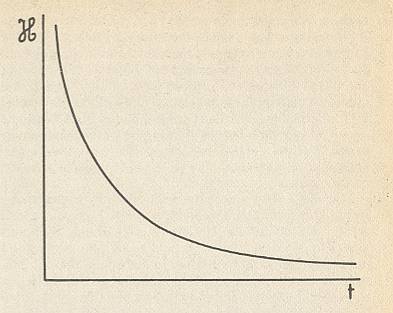
Figure above : Time evolution of the H quantity corresponding to the Ehrenfest model. This quantity decreases monotonously and vanishes for long times.
(After PRIGOGINE & STENGERS, 1985)
The H quantity varies uniformly with time, as does the entropy of an isolated system. It is true that H decreases with time, while the entropy S increases, but that is a matter of definition : H plays the role of minus S ( The difference between the two is that entropy is a macroscopic quantity [like, for instance, temperature], while H stems from a microscopic [involving molecules and atoms] consideration).
where the summation sign refers to all what comes after it.
We will now explain this formula.
To do this we first consider the Ehrenfest model.
Let us say there are 100 marbles (N = 100). These marbles can be distributed over the two boxes A and B.
When there is equilibrium there are 50 marbles in A and 50 marbles in B. So there is a fifty-fifty chance that the marble that we choose is in box A, and a fifty-fifty chance that it is in box B.
So Peq[A] = Peq[B] = 50 /100 = 1/2.
Now say that at time t there are 20 marbles in box A and (thus) 80 in B.
First we look at box A (where, in the discussion, we use a point (.) it means "times" (x), except where it is evidently a decimal point).
The probability that a chosen marble turns out to be in A is : 20/100, which is 1/5.
So P[A,t] = 1/5.
Then P[A,t] / Peq[A] is (1/5)/(1/2) = 2/5.
log ( P[A,t] / Peq[A] ) is then log (2/5) = -0.92 (In all our computations we use the natural logarithm) .
P[A,t] . {log (P[A,t] / Peq[A] } then is (1/5)(-0.92) = -0.18.
Now we look at box B.
The probability that a chosen marble turns out to be in box B is : 80/100, which is 4/5.
So P[B,t] = 4/5 (and thus indeed P[A,t] + P[B,t] = 1, which is a 100% probability).
Then P[B,t] / Peq[B] is (4/5)/(1/2) = 8/5.
log ( P[B,t] / Peq[B] ) is then log (8/5) = 0.47 .
P[B,t] . {log ( P[B,t] / Peq[B] } then is (4/5)(0.47) = 0.38.
We must now add (according to the summation sign in the formula) the results of the two boxes : -0.18 + 0.38 = 0.20 .
So the H value for time t is 0.20 .
When the system is in equilibrium P[A,t] = P[B,t] = Peq[A] = Peq[B], and then
log (P[A,t] / Peq[A] ) = log ( P[B,t] / Peq[B] ) = log 1 = 0.
Therefore P[A,t].0 (i.e. P[A,t] times zero) is 0.
And also P[B,t].0 = 0.
And so P[A,t].0 + P[B,t].0 = 0.
So the H value is 0 when the system is in equilibrium.
Let's give a second example, that is to say a different distribution of the 100 marbles between the two boxes A and B.
Again Peq[A] = Peq[B] = 50 /100 = 1/2.
First we look at box A (where, in the discussion, we use a point (.) it means "times" (x), except where it is evidently a decimal point).
The probability that a chosen marble turns out to be in A is : 10/100, which is 1/10.
So P[A,t] = 1/10.
Then P[A,t] / Peq[A] is (1/10)/(1/2) = 1/5.
log ( P[A,t] / Peq[A] ) is then log (1/5) = -1.61 .
P[A,t] . {log (P[A,t] / Peq[A] } then is (1/10)(-1.61) = -0.16.
Now we look at box B.
The probability that a chosen marble turns out to be in box B is : 90/100, which is 9/10
So P[B,t] = 9/10 (and thus indeed P[A,t] + P[B,t] = 1, which is a 100% probability).
Then P[B,t] / Peq[B] is (9/10)/(1/2) = 9/5.
log ( P[B,t] / Peq[B] ) is then log (9/5) = 0.59 .
P[B,t] . {log ( P[B,t] / Peq[B] } then is (9/10)(0.59) = 0.53.
We must now add (according to the summation sign in the formula) the results of the two boxes : -0.16 + 0.53 = 0.37 .
So the H value for time t is 0.37 .
Let's give a third example, that is to say yet another distribution of the 100 marbles between the two boxes A and B.
Again Peq[A] = Peq[B] = 50 /100 = 1/2.
First we look at box A (where, in the discussion, we use a point (.) it means "times" (x), except where it is evidently a decimal point).
The probability that a chosen marble turns out to be in A is : 0/100, which is 0.
So P[A,t] = 0.
Consequently P[A,t] . {log (P[A,t] / Peq[A] } then is 0.
Now we look at box B.
The probability that a chosen marble turns out to be in box B is : 100/100, which is 1.
So P[B,t] = 1 (and thus indeed P[A,t] + P[B,t] = 1, which is a 100% probability).
Then P[B,t] / Peq[B] is (1)/(1/2) = 2.
log ( P[B,t] / Peq[B] ) is then log (2) = 0.69 .
P[B,t] . {log ( P[B,t] / Peq[B] } then is (1)(0.69) = 0.69.
We must now add (according to the summation sign in the formula) the results of the two boxes : 0 + 0.69 = 0.69 .
So the H value for time t is 0.69 .
Let's give a fourth (and last) example, that is to say yet another distribution of the 100 marbles between the two boxes A and B.
Again Peq[A] = Peq[B] = 50 /100 = 1/2.
First we look at box A.
The probability that a chosen marble turns out to be in box A is : 50/100, which is 1/2.
So P[A,t] = 1/2 .
Then P[A,t] / Peq[A] is (1/2)/(1/2) = 1.
log ( P[A,t] / Peq[A] ) is then log (1) = 0.
P[A,t] . {log (P[A,t] / Peq[A] } then is (1/2)(0) = 0.
Now we look at box B.
The probability that a chosen marble turns out to be in box B is : 50/100, which is 1/2.
So P[B,t] = 1/2 (and thus indeed P[A,t] + P[B,t] = 1, which is a 100% probability).
Then P[B,t] / Peq[B] is (1/2)/(1/2) = 1.
log ( P[B,t] / Peq[B] ) is then log (1) = 0.
P[B,t] . {log ( P[B,t] / Peq[B] } then is (1/2)(0) = 0.
We must now add (according to the summation sign in the formula) the results of the two boxes : 0 + 0 = 0 .
So the H value for time t -- which here is the equilibrium time -- is 0 .
Let us summarize these four results :
| Distribution | H value |
| 0 --- 100 | 0.69 |
| 10 --- 90 | 0.37 |
| 20 --- 80 | 0.20 |
| 50 --- 50 | 0 |
We see that while the nivellation increases the H value decreases. Its limit is 0.
Finally, we calculate the H value generally :
P[B,t] = (N-n)/N = 1 - (n/N) .
P[B,t] / Peq[B] = (1 - (n/N)) / (1/2) = 2 - (2n/N) .
log ( P[B,t] / Peq[B] ) = log (2 - (2n/N)).
P[B,t] . log ( P[B,t] / Peq[B] ) = {1 - (n/N)}{log (2 - (2n/N))}.
We must now add (according to the summation sign in the formula) the results of the two boxes : (n/N)(log (2n/N)) + {1 - (n/N)}{log (2 - (2n/N))} .
So the (general) H value for time t in the Ehrenfest model is
(n/N)( log ( 2n/N)) + {1 - (n/N)}{ log (2 - ( 2n/N))} .
We will now compute H values for a more generalized system, that is for a system consisting of more than two boxes.
So at equilibrium Peq[A] = Peq[B] = Peq[C] =, etc. is equal to 1/8 ,
where the eight boxes are labelled by letters :
The eight particles allow for many different distributions, for example 6 particles in one box and 2 in another. The definition of the H quantity (i.e. its formula) does not distinguish between where in the sequence of boxes A, B, C, D, E, F, G, H the 2 particles are and where the 6 particles. So, for example, the follwing distributions are equivalent :
It is just about the numerical 'diffusion' of the number of particles representing the total.
When we compute the H values belonging to the corresponding distributions, we again follow the formula given above , that is to say we compute :
P[X,t] (where X is either A, or B, or, C, etc.),
Peq[X] (which is 1/8),
P[X,t] / Peq[X],
log ( P[X,t] / Peq[X] ), and
P[X,t] . log ( P[X,t] / Peq[X] ). This result is to be obtained for each box. The eight results will then be added together, yielding the H value for time t .
(When a point (.) is used, it means "times" (x), except where it is evidently a decimal point).
We will now consider some possible distributions of the eight particles between the eight boxes A, B, C, D, E, F, G, H, and compute the corresponding H values. To see these computations click HERE . The results of the computations are summarized in the following overview :
Figure above : Some possible distributions ('diffusion states') of eight particles between eight boxes, and their corresponding H values. We see that while the leveling-out increases, the H value decreases.
The next Figure is the same as the previous one, but miniaturized to obtain a direct overview.
Figure above : Same as previous Figure, but miniaturized. We can clearly see that when the distribution diffuses, the H value decreases.
Strongly heterogeneous, i.e. unequal, distributions.
The less uniformity a given distribution of particles in a container has, the more information it possesses ( The container can be imagined to be partitioned into a (large) number of separate regions, without walls separating these regions, i.e. the container is (only) mentally divided into those regions, allowing to assess the degree of uniformity of the distribution of particles contained in it). And the less uniformity there is, the higher the corresponding H value.
Let us give two examples of such a high degree of heterogeneity (low degree of uniformity or homogeneity).
Suppose we have a container which we mentally have divided into 10000 non-overlapping regions, and suppose there are 1000000 particles, and that at time t they all are present in one such region k , while there is none in the other regions. Let us compute the H value pertaining to this distribution :
If each region were to contain 100 particles, then we would have the equilibrium distribution.
So Peq[k] = 100 / 1000000 = 1/10000 .
Region k
P[k,t] = 1000000 / 1000000 = 1 .
Peq[k] = 1/10000 .
P[k,t] / Peq[k] = 1 / (1/10000) = 10000 .
log ( P[k,t] / Peq[k] ) = log 10000 = 9.210 (as always, the natural logarithm).
P[k,t] . { log ( P[k,t] / Peq[k] ) } = (1)(9.210) = 9.210 .
For each other region r we have :
P[r,t] = 0/1000000 = 0 .
So P[r,t] . { log ( P[r,t] / Peq[r] ) } = (0) . { log ( P[r,t] / Peq[r] ) } = 0 .
So the H value of this distribution
(106 00000000000000000000000000000 . . . 00000000 (ten thousand minus one zero's)) is :
9.210 + 0 + 0 + 0 + . . . + 0 = 9.210 .
We should compare this value with the value 2.08 (obtained earlier) that pertains to the distribution 8 0 0 0 0 0 0 0 .
As a second example of a strongly heterogeneous distribution we could suppose that we have a container that is mentally divided into 1000000000 = 109 regions, and that we have 1011 particles, and that at time t they all are present in one such region k , while there is none in the other regions. Let us compute the H value pertaining to this distribution :
If each region were to contain 100 particles, then we would have the equilibrium distribution.
So Peq[k] = 100/1011 = 1/109 .
Region k
P[k,t] = 1011 / 1011 = 1 .
Peq[k] = 1/109 .
P[k,t] / Peq[k] = 1 / (1/109 ) = 109 .
log ( P[k,t] / Peq[k] ) = log 109 = 20.723 (as always, the natural logarithm).
P[k,t] . { log ( P[k,t] / Peq[k] ) } = (1)(20.723) = 20.723 .
For each other region r we have :
P[r,t] = 0/1011 = 0 .
So P[r,t] . { log ( P[r,t] / Peq[r] ) } = (0) . { log ( P[r,t] / Peq[r] ) } = 0 .
So the H value of this distribution
(1011 00000000000000000000000000000 . . . 00000000 (109 minus one zero's)) is :
20.723 + 0 + 0 + 0 + . . . + 0 = 20.723 .
We should compare this value with the value 9.210 pertaining to the previous distribution, and the value 2.08 (obtained earlier) pertaining to the distribution 8 0 0 0 0 0 0 0 .
We see that a very low uniformity corresponds to a high H value, and it is to be expected that distributions that tend to be infinitely heterogeneous have a H value that approaches to infinity. Such distributions contain a large amount of information. And as soon as this information becomes (in the limit) infinite, they are not realizable in nature. But it should be clear that already a distribution with a finite amount of information is not realizable when this amount exceeds a certain (finite) threshold.
There are other distributions (we're still talking about spatial distributions) that seem to be less uniform than certain others, but have the same H value nevertheless. Let us give a few examples.
Box A.
P[A,t] = 8/8 = 1 .
Peq[A] = 1/8 .
P[A,t] / Peq[A] = 1 / (1/8) = 8 .
log ( P[A,t] / Peq[A] ) = log 8 = 2.08 .
P[A,t] . { log ( P[A,t] / Peq[A] ) } = 1 x 2.08 = 2.08 .
Box B.
P[B,t] = 0/8 = 0, so
P[B,t] . { log ( P[B,t] / Peq[B] ) } = 0 .
The same goes for all the remaining boxes ( P[C,t] = 0/8, P[D,t] = 0/8, etc.).
So the H value for this distribution is
2.08 + 0 + 0 + 0 + 0 + 0 + 0 + 0 = 2.08 .
We could wonder what is the case if we still had these eight boxes, but now having, say, 1600 particles (instead of 8), all of them in one box [box A], while none in the other (seven) boxes. At first sight the distribution
seems to be much more uniform (that is, much more homogeneous) than the distribution
but in fact they have the same degree of non-uniformity.
Let us calculate the H value of this last mentioned distribution -- a distribution present at time t -- :
Box A.
P[A,t] = 1600/1600 = 1 .
At equilibrium the 1600 particles are equally distributed between the eight boxes, which means that then each box contains 1600/8 particles.
So Peq[A] = (1600/8)/(1600) = 1/8 .
P[A,t] / Peq[A] = 1 / (1/8) = 8 .
log ( P[A,t] / Peq[A] ) = log 8 = 2.08 .
P[A,t] . { log ( P[A,t] / Peq[A] ) } = 1 x 2.08 = 2.08 .
Box B.
P[B,t] = 0/1600 = 0, so
P[B,t] . { log ( P[B,t] / Peq[B] ) } = 0 .
The same goes for all the remaining boxes ( P[C,t] = 0/8, P[D,t] = 0/8, etc.).
So the H value for this distribution is
2.08 + 0 + 0 + 0 + 0 + 0 + 0 + 0 = 2.08 .
So we see that both distributions have the same H value, and it is now clear what this value actually tells us : Although both distributions have the same H value, the one looks more extreme in the sense of 1600 particles being concentrated in one box, instead of only eight. But if we look to their respective equilibrium distributions, we see that in the case of (a total of) 1600 particles, 200 are crowded in each box, while only one in the case of (a total of) 8 particles :
(equilibrium distribution for 8 particles and eight boxes)
(equilibrium distribution for 1600 particles and eight boxes)
So the higher degree of crowdedness of the 1600 (instead of only eight) particles in one box at time t corresponds to the more crowdedness of 200 (instead of only one) particles in each box at (the time of) equilibrium. And now it is clear that the transition from
We see that the ratio of the number of particles present in each box at the time of equilibrium and the total number of particles that could be crowded up in one box is equal in all cases of eight boxes and whatever (total) number of particles. For our two discussed cases these ratio's were 1/8 and 200/1600 respectively, which are equal.
Generally, when the number of boxes is k , and the total number of particles N (which total number can be crowded in one box), we get :
Number of particles present in each box at the time of equilibrium is N/k ,
and the total number of particles is N,
so the just mentioned ratio is : (N/k) / N = 1/k .
We see that this ratio is independent of the total number of particles distributed between k boxes.
The course of the H function.
It can be shown that the H function (which we obtain when plotting the H values pertaining to successive distributions of particles that become more and more uniform in time) decreases in a uniform fashion, in accordance with the Figure above . This is why H plays the role of -S (i.e. minus S), entropy. The uniform decrease of H has a very simple meaning : It measures the progressive uniformization of the system. The initial information is lost, and the system evolves from "order" to "disorder".
PRIGOGINE & STENGERS note that a Markov process (as exemplified by the Ehrenfest model or by its generalizations) implies fluctuations (See Figure above ). If we would wait long enough we would recover the initial state. However, we are -- with respect to the H function -- dealing with averages. The HM quantity that decreases uniformly is expressed in terms of probability distributions and not in terms of individual events. It is the probability distribution that evolves irreversibly. Therefore, on the level of distribution functions, Markov chains lead to a one-wayness in time.
It is important to dwell a little longer on this point.
A generalized Ehrenfest process is a process of changing (spatial) distributions. Such a distribution is a distribution of particles (of a given set) between imaginary subdivisions of a container. There are a definite number of these subdivisions ('boxes') and a definite number of particles. Further we assume a starting state which represents a clearly inhomogeneous distribution of the particles between these boxes. Now, every, say, second, we take a particle at random from one of the boxes and put it into another box. This changes the distribution of the particles. The just mentioned "at random" means that each particle of the (total) set has exactly the same chance of being taken (and then transferred to another box). This implies that in the case of a box containing relatively many particles there is a correspondingly high probability that a particle is being taken from it (and transferred to another box) as compared to boxes containing only a relatively small number of particles.
When this process proceeds, the system will, with small ups and downs, approach the equilibrium distribution in which every box contains the same number of particles. This is clearly a model for the diffusion of a diluted gas through air (i.e. a gas, say chlorine, that initially found itself localized in a certain part of an air-filled container, diffuses through the air of the container until it becomes evenly spread throughout the volume of this container).
If we follow this diffusion process we see a succession of different distributions. This succession generally tends to go to an equilibrium distribution. But, because the choice of taking a particle (and tranferring it to another box) is random, it can happen that the course to the equilibrium distribution is not smooth. From a given distribution there could follow one or more distributions that are farther away from the equilibrium distribution than was the initial distribution. And these can be followed by other distributions which are closer again to the equilibrium distribution. Of course such a process, seen in this way, cannot carry the arrow of time, because the latter is supposed to be a continuous flow without hops and bumps.
How then can the arrow of time -- so evident at the macroscopic level -- be detected at the microscopic level of diffusing particles? Or, equivalently, can we detect some quantity that smoothly and uniformly changes during this diffusion process ?
Indeed, Boltzmann found such a quantity -- the H quantity. This quantity smoothly and uniformly decreases as time goes by during the diffusion process. It is the smooth and uniform H function. But why is this function smooth and uniform?
At first sight we would expect it not to be uniform : Each distribution (of a number of particles between boxes) corresponds to a definite H value. So when we follow the actual succession of distributions taking place in a diffusion process, and -- as has been said -- taking place with ups and downs, the sequence of corresponding H values will certainly not represent a smooth and uniform succession. This reasoning is, however, false : The H values are computed from probabilities, not from individual events, i.e. it is about averages.
The quantities P[k,t] and Peq[k] which determine the H value of a given distribution are probabilities. P[k,t] is the probability that at time t a particle is taken from box k (and transferred to another box). Say that this probability is 1/8. This does not mean that if we repeat the action of taking a particle at random eight times (while every time putting the particle back into box k if it was taken therefrom), that in one such repeat the particle was taken from box k while in the seven other repeats the particle was taken from some other box. On the contrary, it could happen that in none of these eight repeats (the first included) a particle was taken from box k , or that, in, say, three (of the eight) repeats a particle was taken from that box. So what then does P[k,t] = 1/8 mean? Well, it means that if we repeat the action of taking a particle at random many times (while every time putting the particle back into box k if it was taken therefrom), then the ratio of the total number of particles actually taken from box k and the total number of repeats (including the initial action) approaches 1/8. So when P[k,t] = 1/8, there is a 1/8 chance that a particle is taken from box k at time t . In a large number of repeats approximately 1/8 of them will consist in taking a particle from box k .
In fact this means that when we involve the H function, and thus involve probabilities, we presuppose that we repeat the diffusion process (i.e. the sequence of distributions) many times and then take the average. And now it is clear that a great many of such repeats (each containing irregularities) will, when superimposed upon each other, give a smooth and uniform succession. And such a succession is expressed by the H function.
Why equilibrium lies in the future. The one-wayness of Time.
Having considered (1) partitions associated with the Baker transformation, (2) contracting and dilating fibers in that same Baker transformation, (3) Markov chains , and (4) the H function, we can now present a possible explanation (based on PRIGOGINE & STENGERS, 1984) of why experience always shows (macroscopic) processes to go to equilibrium in the f u t u r e and not in the past.
Let us recapitulate some considerations made earlier, where we introduced contracting and dilating fibers in the Baker transformation. Earlier we gave a Figure showing the evolution of these fibers when going forward (and can read backwards) in time :
and commented on these fibers as follows :
Let us concentrate on the precise difference between contracting and dilating fibers (See Figure above). A system, as unstable as the baker transformation is a system of scattering hards spheres. Here contracting and dilating fibers have a simple physical interpretation.
A contracting fiber corresponds to a collection of hard spheres whose velocities (expressing speed and direction) are randomly distributed in the far distant past (equilibrium in the past), and all (velocities) become parallel in the far distant future (one point in phase space).
A dilating fiber corresponds to the inverse situation, in which we start with parallel velocities (one point in phase space) and go to a random distribution of velocities (equilibrium in the future).
The exclusion of the contracting fibers corresponds to the experimental and observational fact that whatever the ingenuity of the experimenter or the skill of the observer, he will never be able to control or observe the system to produce parallel velocities after an arbitrary number of collisions.
So, in a way, the Second Law of Thermodynamics (Law of ever increasing entropy) acts as a selection principle, excluding the contracting fibers, and thus only admits systems that go to equilibrium in the future (provided they can go their business unimpededly, i.e. spontaneously). Once we exclude contracting fibers we are left with only one of the two possible Markov chains. In other words, the Second Law becomes a selection principle of initial conditions (one such condition is a contracting fiber, while the other is a dilating fiber). Only initial conditions that go to equilibrium in the future are retained.
Now we continue this discussion in order to explain why some initial conditions are allowed by the Second Law and others prohibited.
A contracting fiber and a dilating fiber correspond to two realizations of dynamics, each involving symmetry-breaking and appearing in pairs ( PRIGOGINE & STENGERS, p. 275 of the 1985 Flamingo edition) [ These two realizations can be seen as two solutions, both (and each for itself) satisfying some dynamic equation. Insofar as we have these two solutions, symmetry is not broken. But, as only one of them is realized as the actual outcome of a real-world process, symmetry is broken. ]. The contracting fiber corresponds to equilibrium in the far distant past, the dilating fiber to equilibrium in the future. We therefore have two Markov chains oriented in opposite time directions. And one of these Markov chains is excluded by the Second Law, resulting in one irreversible process.
How is this conclusion compatible with dynamics? In dynamics "information" is conserved, while in Markov chains information is lost (and entropy therefore increases). There is, however, no contradiction (Ibid., p.276). When we go from the dynamic description of the Baker transformation to the thermodynamic description, we have to modify our distribution function. The "objects" in terms of which entropy increases are different from the ones considered in dynamics. The new distribution function corresponds to an intrinsically time-oriented description of the dynamic system (Ibid., p.277).
An infinite entropy barrier separates possible initial conditions from prohibited ones. Because this barrier is infinite it cannot be overcome. The result is an irreversible process. We have to abandon the hope that one day we will be able to travel back into our past.
To understand the origin of this barrier, we return to the expression of the H quantity as it appears in the theory of Markov chains (as given above). We have seen that to each distribution we can associate a number -- the corresponding value of H. We can say that to each distribution corresponds a well-defined information content. The higher the information content, the more difficult it will be to realize the corresponding state. What we are about to show here is that the initial distribution prohibited by the Second Law would have an infinite information content. That is the reason why we can neither realize such a distribution nor find it in nature.
Let us first come back to the meaning of H as presented earlier. We have to subdivide the relevant phase space into sectors or boxes. With each box k we associate a probability Peq[k] at equilibrium as well as a non-equilibrium probability P[k,t]. The H is a measure of the difference between P[k,t] and Peq[k], and vanishes at equilibrium when this difference disappears, i.e. when P[k,t] = Peq[k] :
P[k,t] / Peq[k] = 1 .
log ( P[k,t] / Peq[k] ) = log 1 = 0 .
And because at equilibrium all boxes have this value, the H value is
0 + 0 + 0 + . . . = 0 .
Therefore, to compare the Baker transformation with Markov chains, we have to make more precise the corresponding choice of boxes. For this we again give the Figure showing the generating partition and (some of) the basic partitions of the Baker transformation phase space :
Figure above : Baker transformation applied, from time 0, three times forward and two times backward. The black and white areas can be considered to represent partitions of the phase space. And the partition pertaining to time 0 will be called the generating partition (or standard partition). The remaining partitions (also those beyond the ones drawn) are basic partitions.
Suppose we consider a system at time 2 (see Figure above), and suppose that this system originated at time ti . Then, a result of dynamical theory is that the boxes correspond to all possible intersections among the partitions between time ti and t = 2. If we now consider the Figure above, we see that when ti is receding towards the past (which means that we consider the system -- as it shows itself at time 2 -- being older and older), the boxes will become steadily thinner as we have to introduce more and more vertical subdivisions. This is expressed in the following Figure, where the arrows signify the direction from past to present :
We see indeed that the number of boxes increases in this way from 4 to 32.
Once we have the boxes, we can compare the non-equilibrium probability with the equilibrium probability for each box (i.e. assess these probabilities, and thus being able to compute the H value associated with that (particular) non-equilibrium distribution). In the present case, the non-equilibrium distribution is either a dilating fiber (Sequence A in the next Figure) or a contracting fiber (Sequence C in next Figure).
Figure above : Dilating (sequence A) and contracting (sequence C) fibers cross various numbers of the boxes which subdivide a Baker transformation phase space. All "squares" on a given sequence refer to the same time, t = 2, but the number of boxes subdividing each square depends on the initial time ti of the system, i.e. the number of boxes depends on how far back into the past the origin of the system lies. The fiber (red), as drawn in both sequences, is supposed to represent where in phase space, at time 2, the system might be. Here, in each case -- contracting fiber, dilating fiber -- the "where" refers to only one coordinate : with respect to the contracting fiber it is the horizontal coordinate, whereas with respect to the dilating fiber it is the vertical coordinate.
The important point to notice is that when ti is receding to the past (i.e. the system, seen at time 2, is considered to be older and older) the d i l a t i n g fiber occupies an increasing large number of boxes : for ti = 1 it occupies one box, for ti = 0 it occupies 2 boxes, for ti = -1 it occupies 4 boxes, for ti = -2 it occupies 8 boxes, and so on, whereas the c o n t r a c t i n g fiber occupies 4 boxes for all ti's.
where log is the natural logarithm (often written as ln ).
If we have, say, 12 boxes, A, B, C, D, E, F, G, H, I, J, K, L, and, say, 12 marbles, such that each of the first four boxes, that is, A, B, C, and D, contains three marbles, while the other boxes containe none, then we can compute the H value associated with this particular distribution. See next Figure.
Figure above :
Top : The described distribution of 12 marbles between 12 boxes.
Bottom : The distribution when the system is in equilibrium.
To compute the H value, we must first calculate the probability of finding a marble in a given box. This probability means the following :
P[A, t] = 3/12
Peq[A] = 1/12
P[A, t] / Peq[A] = (3/12)/(1/12) = 3.
log (P[A, t] / Peq[A] ) = log 3 = 1.10
P[A, t] . log (P[A, t] / Peq[A] ) = (3/12)(1.10) = 0.28 .
In the same way we have for box B 0.28
for box C 0.28
and for box D 0.28
Because for the remaining boxes P[X, t] = 0, which is a factor in the formula, we get for each of these remaining boxes 0 .
Summation (according to the summation sign of the formula) gives :
0.28 + 0.28 + 0.28 + 0.28 + 0 + 0 + 0 + 0 + 0 + 0 + 0 + 0 = 1.12
which is the H value for this distribution.
In order to place the above discussed contracting or dilating fibers into the present context (where H values are calculated), we will now interpret the marbles as representing the dynamical system in its phase space. The fact of allowing -- in our example -- more than one marble in a box (which now is a region of phase space) expresses the ability of the area representing the dynamical system (in phase space) to get smeared out all over phase space as the system proceeds. When the system is represented by fibers, phase space can become filled up, either in (i.e. when going to) the past or in the future, as the Figure given above shows.
We can now redraw our distribution (initially a distribution of marbles among boxes) as follows :
In this new drawing we do not have marbles anymore, but a fiber representing a dynamical system in phase space. And this fiber can increase or decrease in length (not in width, its width is supposed to be zero). Of course we must now redraw this further such that we obtain a square phase space in which the dynamical system is represented probabilistically by a fiber. And this brings us fully back to the mentioned Figure where a dilating or contracting fiber statistically represents the system in phase space :
In the next Figure the auxiliary lines are removed (leaving only the fibers [black] in phase space) :
Figure above : Development of contracting fiber (top sequence, red arrows) and dilating fiber (bottom sequence, blue arrows) in the Baker transformation.
In order to interpret our system (the Baker transformation) in terms of Markov chains, and thus also in terms of the associated H function (which evaluates Markov chains in terms of probabilities), we must divide the phase space into boxes, and consider the probability that at some specified point in time the system will be found in a given box. These boxes, dividing phase space, are provided in a natural and objective way by the above described basic partitions and their possible superpositions. Once we have the boxes, we can show why the Second Law prohibits contracting fibers (i.e. prohibits equilibrium in the far distant past) and only allows dilating fibers (equilibrium in the future). For this we must first clarify the exact status of these partitions and their possible superpositions. This will be done by using the concept of operators as they are already used in quantum mechanics, but will now also be used in the present context, that is to say in the context of classical dynamics.
P : Vperp ==> Vperp , which thus is 1.Vperp ,
for that is just the mathematical way of saying that this state is unchanged by the action of the polariser. On the other hand, for the second state ( Vpar , polarization parallel to the optical axis) we get :
P : Vpar ==> 0 , which is thus 0.Vpar ,
for that is just the mathematical statement that the polariser extinguishes this state.
Both expressions illustrate the notion of an operator, namely by the operator P with eigenfunctions Vperp and Vpar and eigenvalues 1 and 0 respectively.
From all this it follows that to each operator there corresponds an ensemble, a 'reservoir' of numerical values. This ensemble forms its 'spectrum'. This spectrum is discrete when the eigenvalues form a discrete series. There exists, for instance, an operator with all the integers 0, 1, 2, . . . as eigenvalues. A spectrum may also be continuous -- for example, when it consists of all the numbers between 0 and 1.
Now we must shortly discuss the concept of superposition of eigenfunctions (or eigenstates), in order to illucidate the superposition of partitions of phase space (resulting in boxes), discussed above. We must take this from quantum mechanics, where superposition of states plays a conspicuous role.
A quantum system, all by itself, developes according to the Schrödinger Equation.
Whatever we can make of this equation, there is no denying that it is a differential equation, not so very different in its way from the differential equations that Newton and Maxwell had used when they had created the fundamental basis of classical physics. To be sure there are some differences. Classical physics tends to express things in terms of second order differential equations, that is ones involving the rate of change of a rate of change (like, for instance, acceleration, which is a rate of change of speed, while speed itself is a rate of change of position), whilst the Schrödinger equation is first order -- it just incorporates a simple rate of change. However, the similarities are more striking than the differences. The great thing about differential equations is that they produce nice smoothly continuous change in the quantities they describe. There is, therefore, none of the fitful air of discontinuity about the Schrödinger equation which we have come to associate with the quantum world. How then do we get these discontinuities from such an equation?
If a quantum mechanical system is left to go its own business without interference, the Schrödinger equation will take care of its development. All will be smooth and determined. However, the act of measurement, of actually observing the system from the outside, involves a traumatic intervention. It is this act which introduces a probabilistic element and discontinuity in the system's experience. When not disturbed, an electron, for instance, is, with respect to where it is, in a state of superposition of position. It is only when we put to it the rude experimental question "where are you?" that it is forced to make a sharp 'choice' between positional possibilies (such as 'here', or 'there'). Up to that moment it can be in a state evolving smoothly according to the Schrödinger equation, gently and continuously trimming the balance between 'here' and 'there'. At the moment of experimental interrogation it must 'choose' the stark alternative of one or the other. A measurement involves the registration of the result by some macroscopic device operating in the world of everyday experience. Originally the electron was in a state of uncertain position (uncertain in an ontological sense, i.e. not solely because of our ignorance) : it might be 'here' or it might be 'there', with certain probabilities. However, once its position has been determined it is in a totally different state, one of definite position : The electron originally was not in an eigenstate of position but in some superposition of such states. After the act of measurement it finds itself in an eigenstate of position corresponding to the eigenvalue which is the result of that particular measurement.
We encounter a similar example of this happening when speaking about the transmission of light through a polariser. The crystal acts an an analyser which ascertains whether or not a given photon (i.e. a particle of light) has polarization perpendicular to the optical axis of the crystal. The photons which approached the crystals were in a state which was a superposition of that state of polarization together with the state of polarization parallel to the optical axis. The transmitted beam, i.e. the bean that comes out of the crystal, consists only of photons with the perpendicular polarization. Being let through the crystal is tantamount to a polarization measurement and it changes the photon's polarization state in this discontinuous way. Every act of (quantum) measurement has this character of entailing instant change. Beforehand our system is not in general in an eigenstate of the observable we are intending to measure but rather it is a superposition of such states. Afterwards the system is in that particular eigenstate, selected from the original superposition, which (eigenstate) corresponds to the eigenvalue actually obtained as the result of that measurement. In the jargon of quantum mechanics this discontinuous change is called the collapse of the wavepacket. The idea is that probability, which was originally spread out in a wavefunction (or packet) covering (with regard to position) 'here', 'there' and perhaps 'everywhere', is now all concentrated 'here'. It has collapsed in on itself.
From a historical point of view, the introduction of operators is linked to the existence of energy levels in the submicroscopic world, but today operators have applications even in classical physics. This implies that their significance has been extended beyond the expectations of the founders of quantum mechanics. Operators now come into play as soon as, for one reason or another, the notion of a dynamic trajectory has to be discarded, and with it, the deterministic description a trajectory implies.
I hope that now the idea of operators, eigenfunctions (or eigenstates), eigenvalues, and superposition of states is reasonably clear.
We now return to the above discussed Baker transformation and its relation to Markov chains, and with it to the associated H function describing such chains in terms of probability. In order to do so we had to divide the phase space into boxes, and must determine the probability that the system is present in a given box. This we do with partitions, which evolve from a generating or standard partition, by applying the Baker transformation to the generating partition :
Figure above : Baker transformation applied, from time 0, three times forward and two times backward. The black and white areas can be considered to represent partitions of the phase space. And the partition pertaining to time 0 will be called the generating partition (or standard partition). The remaining partitions (also those beyond the ones drawn) are basic partitions.
Every basic partition represents the internal time T of the system determined by the number of times we must apply the Baker transformation to the generating partition to obtain a given basic partition. The black areas indicate where precisely the system might be in phase space.
Now we can say the following :
This internal time, which we shall denote by T, is in fact an operator like those introduced in quantum mechanics. Indeed, an arbitrary partition of the square (representing the phase space of the Baker transformation) does not have a well-defined time, but only an 'average' time corresponding to the superposition of the basic partitions out of which it is formed (PRIGOGINE & STENGERS, p.272 (note) of the 1985/6 Flamingo edition).
So the basic partitions must be eigenfunctions or eigenstates of the internal time operator T, whilst the operator's eigenvalues are the number of times the Baker transformation had to be applied to the generating partition to reach a given basic partition. A superposition of basic partitions is the superposition of eigenfunctions or eigenstates. The basic partitions and their superpositions (obtainable by geometrically superimposing the (relevant) basic partitions) constitute the boxes of the phase space of the Baker transformation, and these boxes have now obtained a natural and objective status.
We will now continue our discussion that will establish the reason why the Second Law of Thermodynamics prohibits certain initial states and allows others. In fact it is about the states either represented by a contracting fiber or by a dilating fiber. Such a fiber indicates where the system (the Baker transformation and the geometrical points on which it acts) might be in phase space, or, said differently, in what state the system is in.
We were considering this system at internal time t = 2 (see Figure above) characterized by a basic partition consisting of four horizontal boxes (two of them black) stacked on top of each other. We here only look to the partitions themselves, as dividing phase space into boxes, not to the black or whiteness of the boxes : The blackness initially indicated where the system could be in phase space. Now, however, we have segregated two aspects of this by means of letting the system be represented by a line (fiber) instead of by an area, that is to say either by a vertical fiber ('contracting fiber') or by a horizontal fiber ('dilating fiber'). Originally the partitions showed that out of the unstable dynamic process we obtain two Markov chains (discussed above ), one reaching equilibrium in the future, one in the past. By introducing fibers (See Figure given earlier ) we have segregated these two chains (Both renderings of the Baker transformation, the one with areas and the one with fibers, are not Markov chains, but can be mapped onto them).
To pick up our earlier discussion, we have used the basic partitions to indicate the internal time of the system, that is to say the system's intrinsic age, while this is contrasted with the system's actual age, i.e. how far back into the past the origin of the system lies (the system's extrinsic age).
A good analogy for this can be provided by cities : If the city of New York were built at the time when Pompei was built, then New York's intrinsic age is that of a very young city, despite its actual age, while Pompei's intrinsic age is that of a very old city despite the fact that it has been (supposedly) built in the same period as was New York.
Modern Rome, on the other hand, has no intrinsic or internal age, since it contains buildings of all eras between that of Pompei and the present era. The age of Rome is a superposition of many ages.
Before we continue to compare the Baker transformation with Markov chains, it is important to realize that, like the Clock Doubling Process (discussed in Part XXIX Sequel-27), the Baker transformation is a mathematical prescription that tells us whereto a given point at a given location must move. In fact this prescription refers to every point of a given area, and then we follow the fate of one point, while applying the prescription again and again. The present state of the system is then nothing more than the present location of the point (which had been followed). From this it is clear that the Baker transformation (as is the Clock Doubling system), when geometrically depicted, is, as a system, at the same time also its phase space.
When we, while repeating the Baker transformation, follow some one area (instead of some one point), then this area tends to diffuse or expand, until it finally is everywhere in phase space. And because, with respect to the Baker transformation (and Clock Doubling), the phase space is the same as the system itself, we can indeed interpret the expansion of the initial area (i.e. a non-point), whether it be a fiber or a genuine area, as a diffusion of some substance (like ink [as PRIGOGINE & STENGERS indeed refer to in precisely this context] ), which reaches equilibrium when that substance has spread out all over the available space.
Now, we were looking at the system, represented statistically by either a contracting fiber or a dilating fiber (in fact both, but separately depicted) at internal time t = 2 (See Figure given earlier ). The basic partition corresponding to internal time t = 2 divides the phase space into four horizontal boxes. If we now let the system's origin (indicated as ti , initial time) recede further and further into the past, the system then has no well-defined internal age anymore. Its age is now a superposition of many ages, and thus a superposition of many basic partitions (namely the intersection of all those partitions between ti and t = 2 ), resulting in an increase in the number of boxes :
Figure above : Dilating (sequence A) and contracting (sequence C) fibers cross various numbers of the boxes which subdivide a Baker transformation phase space. All "squares" on a given sequence refer to the same time, t = 2, but the number of boxes subdividing each square depends on the initial time ti of the system, i.e. the number of boxes depends on how far back into the past the origin of the system lies. The fiber (red), as drawn in both sequences, which is a line, not an area, is supposed to represent where in phase space, at time 2, the system might be. Here, in each case -- contracting fiber, dilating fiber -- the "where" refers to only one coordinate : with respect to the contracting fiber it is the horizontal coordinate, whereas with respect to the dilating fiber it is the vertical coordinate.
We see that when ti is receding to the past, the dilating fiber occupies an increasing large number of boxes (Sequence A of the above Figure).
Let us compute some H values for some boxes in the sequence of the dilating fiber (sequence A of the above Figure, which, of course, is only a segment of the total sequence [where ti is receding more and more into the past] ).
We refer to the position in phase space where the system is -- indicated by the fiber -- in terms of boxes, i.e. which boxes contain part of the fiber. Statistically the system is in every box that contains a part of the fiber. So for the initial time ti = 1, and investigating the case of the dilating fiber, we have a corresponding partition that is a superposition (intersection) of the basic partitions between ti = 1 and t = 2, so we have :
which we take to be equivalent to
for the non-equilibrium distribution.
While for the equilibrium distribution we have :
When, at (internal) time t = 2 the system were in equilibrium, the phase space would then be fully filled up with horizontal fibers (at most infinitesimal distances between them).
The fact that the number of 'marbles' in the equilibrium distribution is larger than in the non-equilibrium distribution, expresses the fact that the area indicating where the system is in phase space smears out upon approaching equilibrium till it is present in every box.
If we index the boxes with the letters A, B, C, D, from the top down, we can compute the H value for this distribution acording to the formula given above :
P[A, 2] = 0/1 = 0 .
And because P[A, 2] is a factor in the formula we get 0.
The same holds for the boxes C and D.
P[B, 2] = 1/1 = 1 .
Peq[B] = 1/4 .
P[B, 2] / Peq[B] = 1/(1/4) = 4 .
log ( P[B, 2] / Peq[B] ) = log 4 = 1.39 .
P[B, 2] . log ( P[B, 2] / Peq[B] ) = (1)(1.39) =
1.39 .
Summation (according to the summation sign of the formula) of the results for the four boxes gives 0 + 1.39 + 0 + 0 = 1.39 which is the H value for this (non-equilibrium) distribution.
Now we consider ti to be receded further into the past : ti = 0.
where we name the eight boxes a, b, c, d, e, f, g, h.
Again we compute the H value for this (non-equilibrium) distribution :
P[a, 2] = 0/2 = 0
And because P[a, 2] is a factor in the formula we get 0.
The same holds for the boxes b, e, f, g, and h.
P[c, 2] = 1/2
Peq[c] = 1/8 .
P[c, 2] / Peq[c] = (1/2)/(1/8) = 4 .
log ( P[c, 2] / Peq[c] ) = log 4 = 1.39 .
P[c, 2] . log ( P[c, 2] / Peq[c] ) = (1/2)(1.39) =
0.70 .
P[d, 2] = 1/2
Peq[d] = 1/8 .
P[d, 2] / Peq[d] = (1/2)/(1/8) = 4 .
log ( P[d, 2] / Peq[d] ) = log 4 = 1.39 .
P[d, 2] . log ( P[d, 2] / Peq[d] ) = (1/2)(1.39) =
0.70 (as always, rounded off to two digits after the decimal point).
Summation (according to the summation sign of the formula) of the results for the eight boxes gives 0 + 0 + 0.70 + 0.70 + 0 + 0 + 0 + 0 = 1.39 which is the H value for this (non-equilibrium) distribution.
Now we consider ti to be receded still further into the past : ti = -1.
where we name the sixteen boxes a, b, c, d, e, f, g, h, i, j, k, l, m, n, o, p.
Again we compute the H value for this (non-equilibrium) distribution :
P[a, 2] = 0/4 = 0
And because P[a, 2] is a factor in the formula we get 0.
The same holds for the boxes b, c, d, i, j, k, l, m, n, o, and p.
P[e, 2] = 1/4
Peq[e] = 1/16 .
P[e, 2] / Peq[e] = (1/4)/(1/16) = 4 .
log ( P[e, 2] / Peq[e] ) = log 4 = 1.39 .
P[e, 2] . log ( P[e, 2] / Peq[e] ) = (1/4)(1.39) =
0.35 .
P[f, 2] = 1/4
Peq[f] = 1/16 .
P[f, 2] / Peq[f] = (1/4)/(1/16) = 4 .
log ( P[f, 2] / Peq[f] ) = log 4 = 1.39 .
P[f, 2] . log ( P[f, 2] / Peq[f] ) = (1/4)(1.39) =
0.35 .
P[g, 2] = 1/4
Peq[g] = 1/16 .
P[g, 2] / Peq[g] = (1/4)/(1/16) = 4 .
log ( P[g, 2] / Peq[g] ) = log 4 = 1.39 .
P[g, 2] . log ( P[g, 2] / Peq[g] ) = (1/4)(1.39) =
0.35 .
P[h, 2] = 1/4
Peq[h] = 1/16 .
P[h, 2] / Peq[h] = (1/4)/(1/16) = 4 .
log ( P[h, 2] / Peq[h] ) = log 4 = 1.39 .
P[h, 2] . log ( P[h, 2] / Peq[h] ) = (1/4)(1.39) =
0.35 .
Summation (according to the summation sign of the formula) of the results for the sixteen boxes gives 0 + 0 + 0 + 0 + 0.35 + 0.35 + 0.35 + 0.35 + 0 + 0 + 0 + 0 + 0 + 0 + 0 + 0 = 1.39 which is the H value for this (non-equilibrium) distribution.
Now we consider ti to be receded still further into the past : ti = -2.
where we name the thirty-two boxes a, b, c, d, e, f, g, h, i, j, k, l, m, n, o, p, q, r, s, t, etc.
Again we compute the H value for this (non-equilibrium) distribution :
P[a, 2] = 0/8 = 0
And because P[a, 2] is a factor in the formula we get 0.
The same holds for all the boxes except the boxes i, j, k, l, m, n, o, and p.
P[i, 2] = 1/8
Peq[i] = 1/32 .
P[i, 2] / Peq[i] = (1/8)/(1/32) = 4 .
log ( P[i, 2] / Peq[i] ) = log 4 = 1.39 .
P[i, 2] . log ( P[i, 2] / Peq[i] ) = (1/8)(1.39) =
0.17 .
The same value is obtained for the boxes j, k, l, m, n, o, and p.
Summation (according to the summation sign of the formula) of the results for the thirty-two boxes gives 0 + 0 + 0 + 0 + 0 + 0 + 0 + 0 + 0.17 + 0.17 + 0.17 + 0.17 + 0.17 + 0.17 + 0.17 + 0.17 + 0 + 0 + 0 + 0 + 0 + 0 + 0 + 0 + 0 + 0 + 0 + 0 + 0 + 0 + 0 + 0 = 1.39 which is the H value for this (non-equilibrium) distribution.
(8 x 0.17 is of course 1.36, but this small discrepancy is the result of rounding off : We had log 4 = 1.39, then we had to multiply it with 1/8, and then multiply the result by 8, and this results in 1.39 again).
From the above it is clear that the H value remains the same (1.39) and (remains) finite, when ti recedes further and further into the past. So by considering the system at time t = 2 being older and older does not entail unacceptable consequences, and the same goes for all times t : Any distribution represented by a dilating fiber involves a finite amount of information (a finite H value).
Now we will investigate things involving a contracting fiber. We will see that a contracting fiber always remains localized in 4 boxes, whatever ti . Let us see what this means by computing a series of H values pertaining to distributions as we see them in Sequence C of the Figure given earlier .
We first consider, now with respect to the contracting fiber, the case of ti = 1.
The corresponding partition is a superposition (intersection) of the basic partitions between ti = 1 and t = 2, so we have :
where we name the four boxes A, B, C, D.
Again we compute the H value for this distribution :
P[A, 2] = 1/4 .
Peq[A] = 1/4 .
P[A, 2] / Peq[A] = (1/4)/(1/4) = 1.
log ( P[A, 2] / Peq[A] ) = log 1 = 0.
P[A, 2] . log ( P[A, 2] / Peq[A] ) = (1/4)(0) = 0.
This also holds for the boxes B, C, and D.
Summation (according to the summation sign of the formula) of the results for the four boxes gives 0 + 0 + 0 + 0 = 0 which is the H value for this distribution ( this is the lowest possible value of the H function).
Next we consider ti to be receded further into the past : ti = 0.
The corresponding partition is a superposition (intersection) of the basic partitions between ti = 0 and t = 2, so we have :
where we name the eight boxes a, b, c, d, e, f, g, h.
Again we compute the H value for this (non-equilibrium) distribution :
P[a, 2] = 1/4 .
Peq[a] = 1/8 .
P[a, 2] / Peq[a] = (1/4)/(1/8) = 2.
log ( P[a, 2] / Peq[a] ) = log 2 = 0.69 .
P[a, 2] . log ( P[a, 2] / Peq[a] ) = (1/4)(0.69) = 0.17
This also holds for the boxes c, e, and g.
P[b, 2] = 0/4 = 0 .
And because P[b, 2] is a factor in the formula we get 0 .
The same holds for the boxes d, f, and h.
Summation (according to the summation sign of the formula) of the results of the eight boxes gives 0.17 + 0.17 + 0.17 + 0.17 + 0 + 0 + 0 + 0 = 0.68 which is the H value for this (non-equilibrium) distribution.
Next we consider ti to be receded still further into the past : ti = - 1.
The corresponding partition is a superposition (intersection) of the basic partitions between ti = - 1 and t = 2, so we have :
where we name the sixteen boxes a, b, c, d, e, f, g, h, i, j, k, l, m, n, o, p.
Again we compute the H value for this (non-equilibrium) distribution :
P[a, 2] = 0/4 = 0 .
And because P[a, 2] is a factor in the formula we get 0 .
The same goes for the boxes c, d, e, g, h, i, k, l, m, o, and p.
P[b, 2] = 1/4 .
Peq[b] = 1/16 .
P[b, 2] / Peq[b] = (1/4)/(1/16) = 4 .
log ( P[b, 2] / Peq[b] ) = log 4 = 1.39 .
P[b, 2] . log ( P[b, 2] / Peq[b] ) = (1/4)(1.39) = 0.35 .
The same goes for f, j, and n.
Summation (according to the summation sign in the formula) of the results of the 16 boxes gives 4 x 0.35 = 1.39 which is the H value for this (non-equilibrium) distribution.
Next we consider ti to be receded still further into the past : ti = - 2.
The corresponding partition is a superposition (intersection) of the basic partitions between ti = - 2 and t = 2, so we have :
where we name the 32 boxes a, b, c, d, e, f, g, h, i, j, k, l, m, n, o, p, q, r, etc.
Again we compute the H value for this (non-equilibrium) distribution :
P[a, 2] = 0/4 = 0 .
And because P[a, 2] is a factor in the formula we get 0 .
The same goes for all the boxes except c, e, f, and g.
P[c, 2] = 1/4 .
Peq[c] = 1/32 .
P[c, 2] / Peq[c] = (1/4)/(1/32) = 8 .
log ( P[c, 2] / Peq[c] ) = log 8 = 2.08 .
P[c, 2] . log ( P[c, 2] / Peq[c] ) = (1/4)(2.08) = 0.52 .
The same goes for the boxes e, f, and g.
Summation (according to the summation sign of the formula) of the results of the 32 boxes gives 4 x 0.52 = 2.08 which is the H value for this (non-equilibrium) distribution.
We can let ti recede still further into the past.
So we consider now ti = - 3.
And, as seen in the Figure above, the corresponding partition is a superposition (intersection) of the basic partitions between ti = - 3 and t = 2, so we have :
where we name the 64 boxes a, b, c, d, e, f, g, h, i, j, k, l, m, n, o, p, q, r, etc.
Again we compute the H value for this (non-equilibrium) distribution :
P[a, 2] = 0/4 = 0 .
And because P[a, 2] is a factor in the formula we get 0 .
The same goes for all the boxes except c, e, f, and g.
P[c, 2] = 1/4 .
Peq[c] = 1/64 .
P[c, 2] / Peq[c] = (1/4)/(1/64) = 16 .
log ( P[c, 2] / Peq[c] ) = log 16 = 2.77 .
P[c, 2] . log ( P[c, 2] / Peq[c] ) = (1/4)(2.77) = 0.69 .
The same goes for the boxes e, f, and g.
Summation (according to the summation sign of the formula) of the results of the 64 boxes gives 4 x 0.69 = 2.77 which is the H value for this (non-equilibrium) distribution.
If we let ti recede very far into the past, such that, say, ti = -11 , then we have 16384 boxes. But still, the contracting fiber occupies only four of them.
For an empty box e we have
P[e, 2] = 0/4 = 0 .
And because P[e, 2] is a factor in the formula we get 0 .
The same goes for all the empty boxes.
For an occupied box c we have
P[c, 2] = 1/4 .
Peq[c] = 1/16384 .
P[c, 2] / Peq[c] = (1/4)/(1/16384) = 4096 .
log ( P[c, 2] / Peq[c] ) = log 4096 = 8.32 .
P[c, 2] . log ( P[c, 2] / Peq[c] ) = (1/4)(8.32) = 2.08 .
The same goes for the other three occupied boxes.
Summation (according to the summation sign of the formula) of the results of the 16384 boxes gives 4 x 2.08 = 8.32 which is the H value for this (non-equilibrium) distribution.
In concluding with respect to all the above findings, we can now say :
0 ==> 0.68 ==> 1.39 ==> 2.08 ==> 2.77 ==> . . . ==> 8.32 ==>
In this latter case it will be clear that the H value will climb up toward infinity.
This important result -- the dilating fiber involving distributions having a finite H value, however far we let ti recede toward the past, and the contracting fiber involving distributions of which the H value diverges to infinity -- means that the contracting fiber can and will involve distributions with an information content (i.e. how much information is needed to find out which boxes are occupied with the fiber) that approaches to infinity, while this is not so in the case of the dilating fiber. It is this fact that leads to the Second Law of Thermodynamics as a selection principle. Only measures or probabilities, which in the limit of infinite number of boxes, give a finite information or a finite H quantity, can be prepared (in experiments) or observed.
This excludes contracting fibers.
That is to say, already from experience we know that real-world systems (spontaneously) go from order to disorder (at least in terms of high probabilities), or, said equivalently, in real-world (closed) systems the entropy always increases. And this is the Second Law. It acts as a selection principle, which prohibits (spontaneous) processes with equilibrium in the past instead of in the future. See the Figure above , where we see that the contracting fiber entails equilibrium in the past. The Second Law excludes the contracting fiber, and we now know why it does so.
For the same reason we must also exclude distributions concentrated on a single point. Initial conditions corresponding to a single point in unstable systems would again correspond to infinite information and are therefore impossible to realize or observe. Again we see that the Second Law appears as a selection principle.
The information content of a system state can also be present in another (or eventually equivalent?) way, namely when collisions between particles are going to play a significant role. These collisions create correlations between the particles, that is to say a storage of information about earlier events. And also here, the Second Law acts as a selection principle, as we shall see in the next Section ( Which is, as the present Section, based [but supplemented by us] on PRIGOGINE & STENGERS, 1984, Order out of Chaos ).
The Dynamics of Correlations
Considering a dilute gas, we can perform 'thought experiments'. One such thought experiment (which can be converted into a computer simulation) is the reversal of d i r e c t i o n of velocity of all the particles of such a gas at a given instant. From time 0 we follow the evolution of a certain volume of such a dilute gas (which consists of a multitude of moving particles (elastically) colliding now and then). At time t0 we bring about a velocity inversion of each molecule. The gas then returns to its initial state. And for a gas to retrace its past there must be some storage of information. This storage can be described in terms of "correlations" between particles.
These correlations are produced by collisions. In a velocity reversal experiment we have two types of situations : In one, uncorrelated particles enter, are scattered (because of collisions), and correlated particles are produced. In the opposite situation, correlated particles enter, the correlations are destroyed through collisions (which are the initial collisions of the direct process [i.e. before velocity inversion] but with reversed directions ), and uncorrelated particles result.
The two situations differ in the temporal order of collisions and correlations. In the first case, we have "postcollisional" correlations. In the second case, "antecollisional" correlations (or, equivalently, precollisional correlations). With this distinction between ante- and post collisional correlations in mind, let us return to the velocity inversion experiment.
We start at t = 0 , with an initial state corresponding to no correlations between particles. During the time 0 ==> t0 we have a 'normal' evolution. Collisions bring the velocity distribution closer to the Maxwellian equilibrium distribution ( We discussed this distribution at the end [scroll down there if necessary] of the previous document : The Maxwell-Boltzmann Distribution ). Let us reproduce this distribution (for two temperatures) again :
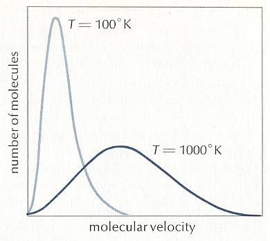
Maxwell-Boltzmann distribution.
Both curves must refer to a gas in equilibrium (only then it has one well-defined temperature (which is the same everywhere in the system)).
From some non-equilibrium state the speed distribution (as it was during that state) evolves to the Maxwell-Boltzmann distribution for a prevailing temperature.
Each individual spatial configuration of particles has -- at equilibrium -- the same probability (only categories of configuration can have different probabilities). Also each direction of movement (of particles) has -- at equilibrium -- the same probability.
The Maxwellian distribution ( = Maxwell-Boltzmann distribution) is a speed distribution, it is not about the directions of molecular movement.
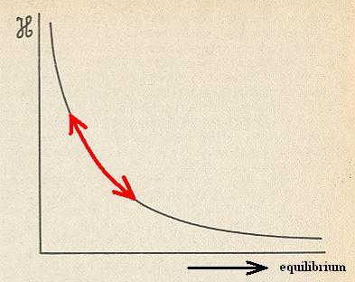
Figure above : H function, here, not as a function of time, but as a function of distance from the state of equilibrium.
The just described inversion experiment 0 ==> t0 ==> 2t0 is here depicted as : First going down along (a part of) the H curve, and then (at time t0 ) going up again. That is to say, while time keeps running forward, the system first moves into the direction of equilibrium, and then moving away from it again.
Such a state of affairs, implying a violation of the Second Law, is quite unsatisfactory.
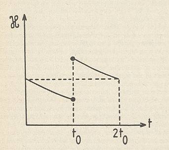
Figure above : Time variation of the H function in the velocity inversion experiment : At time t0 the velocities are inversed and H presents a discontinuity. At time 2t0 the system is in the same state as at time 0 , and H recovers the value it had initially. At all times (except at t0 ), H is decreasing. The important fact is that at time t0 the H quantity takes two different values.
(After PRIGOGINE & STENGERS, 1984 (1986))
In this approach, in contrast with Boltzmann's, the effect of correlations is retained in the new definition of H . Therefore at the velocity inversion point t0 the H quantity will jump (because now we have taken into account the correlations), since we abruptly create abnormal antecollisional correlations that will have to be destroyed later. This jump corresponds to the entropy or information price we have to pay.
Figure above : Dilating and contracting fibers of the Baker transformation interpreted as velocity inversion of each other.
The sequence starts at t = 0 with a distribution (of the system over phase space) with a relatively high H value. Then at time t0 we inverse all velocities. This act, which comes from outside the system, decreases the entropy S of the system and (consequently) increases the H value ( S becomes lower than it initially was, H becomes higher than it initially was, as in the new H function depicted in the Figure above ).
The contracting fiber normally (that is, when we just apply the Baker transformation forwardly (i.e. applying B , and not B-1 ) gets shorter and shorter as time goes by, and thus moves away from equilibrium. Consequently H increases. The system would climb up along the H curve, violating the Second Law. So we must, as is done in the present Figure, reverse the evolution of this fiber (i.e. the contracting fiber), which means applying B-1 , and in this way correctly represent the effect of velocity inversion.
All in all, the velocity inversion experiment starts with a normal evolution (i.e. applying B , and not B-1 ) of the dilating fiber. Then, at time t0 we must do the following : We must find a Baker transformation sequence, (also) originating from a line (a fiber), such that when the evolution of this sequence is reversed (expressing the velocity inversion in our experimment), the sequence neatly goes in the direction of equilibrium, that is to say in the direction of lower H value and higher entropy, and thus not violating the Second Law. And this is satisfied by the contracting fiber.
Suppose we wait a sufficiently long time before making the velocity inversion. The postcollisional correlations would then have an arbitrarily long range (because the particles that collided were given enough time to recede far from each other), and the velocity inversion would then require too high an entropy price, and thus would be excluded. In physical terms this means that the Second Law excludes persistent long-range antecollisional correlations ( That is to say, the long-range postcollisional correlations become, after velocity inversion, long-range antecollisional correlations).
Suppose a film is taken of a large surface of water initially at rest into which a stone is dropped. The reversed film [ which can be seen as a velocity inversion experiment ] will show contracting, circular waves of increasing amplitude. Moreover, immediately behind the highest wave crest, a circular region of undisturbed water will close in towards the centre. This cannot be regarded as a possible classical process. It would demand a vast number of distant coherent generators of waves the coordination of which, to be explicable, would have to be shown, in the film, as originating from one centre [ i.e. the coherence is only understandable if it came from one single spot (centre), because in such a spot, or very small region, it is understandable that there is coherence, which then expands outwards ].Indeed, whatever the technical means, there will always be a distance from the center beyond which we are unable to generate a contracting wave. There are unidirectional processes.
As we have said, the Second Law excludes persistent long-range antecollisional correlations.
The analogy with the macroscopic description of the Second Law is striking. From the point of view of energy conservation, heat and work play the same role (they are just forms of energy), but no longer from the point of view of the Second Law. Briefly speaking, work is a more coherent form of energy and always can be converted into heat, but the inverse is not true (of a given amount of heat only a part can be converted into work). There is on the microscopic level a similar distinction between collisions and correlations. From the point of view of dynamics, collisions and correlations play equivalent roles. Collisions give rise to correlations, and correlations may undo the effect (having taken place earlier) of collisions (because correlations make it possible for the system to run backward). See next Figure.
But there is an essential difference. We can control collisions and produce correlations, but we cannot control correlations in a way that will undo the effects collisions have brought into the system, i.e. we can let transform collisions into correlations, but only short-range correlations can be transformed back into the corresponding collisions again. The transformation of long-range postcollisional correlations into the corresponding long-range antecollisional correlations takes too high an entropy price. It is this essential difference that does not show up in dynamics but that can be incorporated into thermodynamics. In all this, we must -- according to PRIGOGINE & STENGERS -- note that thermodynamics does not enter into conflict with dynamics at any point. It adds an additional, essential element to our understanding of the physical world.
By means of two examples (unstable systems, like the Baker transformation, and the dynamics of correlations) we have shown that real-world processes are intrinsically irreversible. However, they are so irreversible only in a probabilistic sense (as seen in the H function). A Markov chain shows local (with respect to time) small reversals (fluctuations) in its course toward equilibrium (See Figure above ), i.e. small and temporary excursions against the generally prevailing 'leveling out', also when we have only one (instead of two) Markov chain. This means that causality still possesses an intrinsic probabilism, as already found out much earlier.
Having now obtained some overview of thermodynamics and its bearing on the Category of Causality, we will, in the next document concentrate on far-from-equilibrium thermodynamic systems, because they are the systems that generate patterns (branched crystals, organisms, etc.) and are thus relevant for our crystal analogy. So it is also -- or even especially -- in these systems that we must investigate in what way causality is present.
To continue click HERE for further study of the Theory of Layers, Part XXIX Sequel-30.
e-mail :