Cellular Automata

back to homepage

(For a general treatment of Dynamical Systems see the Essay on Dynamical Systems )

Introduction

Cellular Automata form a large family of abstract dynamical systems, and are nowadays well known for their interesting and beautiful performance. On the basis of simple laws they can generate complex patterns and behavior. Although there are many locations on the Internet devoted to cellular automata, for example the most famous Cellular Automaton called " The Game of Life ", it is nevertheless useful to treat them here in a more or less extensive way, in order to make our elaborations of the above mentioned Essay a little more concrete. Of course there are many more types of abstract dynamical systems (like for instance Random Boolean Networks, L-systems, models of continuous dissipative systems, and much more), but Cellular Automata are, it seems, the most transparent and are thus well suited for to begin an elementary treatment of dynamical systems.

Ontological Status of Abstract Systems

Like all abstract dynamical systems, a Cellular Automaton (CA) is, in itself, just a formal system, belonging as such to the Ideal World (of objective, but immaterial patterns). To render it dynamical it should be implemented onto an appropriate material substrate, in order for its deductive patterns to become connected with each other within a time frame. This we can do by choosing a computer as substrate. In this way we get a real-world simulation of a(n) (immaterial) cellular automaton.
Because the Dynamical Law (its 'Rule') is explicitly programmed, we, by doing so, impose (instead of find) certain properties onto the 'elements' of the CA. This explicit programming is necessary, because in a computer simulation we don't in fact have any true system elements that have properties all by themselves, and in this way, i.e. by having these properties, harboring, all by themselves, a dynamical law, governing their interaction.

Remark : In Reality the Dynamical Law follows from certain properties of the system elements, while in a computer simulation we create these properties (of the elements) by explicitly programming of a dynamical law (in our case a CA rule). In this way we transform the elements into (dynamical) system elements.

So a CA (on a computer) is just a simulation (of a certain formal deductive structure). But when we're actually dealing with CA's we always have in mind one or another, albeit sometimes vague, interpretation of them in terms of real-world processes.
Their simplicity and transparency will help us understand those real-world processes.

Cellular Automata (CA)

A Cellular Automaton (CA) is a (computer) simulation of a simple and (inherently) unified discrete dynamical system.
The ' space ' of a Cellular Automaton (CA) (and also of a Boolean Network) consists of a one- or more-dimensional grid of ' cells ' (for instance pixels on a computer screen). These cells are the system elements. So we can have either a row of cells (system elements), making up a one-dimensional CA, or a plane of cells, making up a two-dimensional CA, or a volume of cells, making up a three-dimensional CA, etc. These cells can, each for themselves, be in a certain state, for example white or black (which can be interpreted as, say, on or off, or, as one wishes, as 1 or 0) for two-valued cells, or a cell can have a color chosen from a larger range of possible colors. We call this the cell state. It is the state of every individual cell and so of every individual system element.
The state of the system, the system state, at the point in time t can be defined as : The existing pattern of colors, extending across the whole grid of cells, at the point of time t, (in other words, the configuration of cell states of the grid at time t ).
At every successive discrete point in time the cell state (color) of every cell of the grid is being updated (in other words, at every successive point in time the system state is updated), and this updating, concerning every cell, depends on their own present state (color) and the present state of a predetermined number of neighborhood cells. The precise nature of this dependence is specified in a (chosen) dynamical rule. After every update a new color pattern emerges.
We interpret the dependence of the update (how it will look like) of every cell on the state of the neighborhood cells (including itself) as : interaction.
In a two-dimensional grid we could choose the neighborhood cells of a certain cell C in the following way : The cell C itself plus the cell immediately north of C plus the cell immediately east of C plus the cell immediately south of C plus the cell immediately west of C, and this for every cell of the grid. This grid can be either considered as infinitely extended, or supplied with a special boundary, or a grid which reverts in itself (it then is equivalent to the surface of a donut). When the CA is one-dimensional (thus involving a one-dimensional grid of cells) we have a row of cells. In such a system we could choose a neighborhood for every cell as follows : The cell itself plus its right and left neighbor, and this for every cell of the row, but, we could also, for example, choose : the cell itself plus its two nearest neighbors on the left plus its two nearest neighbors on the right, and this for all the cells of the row.
In CA's, ' time ' is by definition discrete, so it passes with discrete steps : t, t+1, t+2, t+3, etc.
In CA's the interaction of the elements (cells) is local, which means that the update of a cell with respect to a next point in time, is only dependent on the state of one or more cells from its immediate surroundings (immediate neighborhood, this is called a local neighborhood). Moreover for a CA applies that every cell updates itself (undergoes an update) according to one and the same rule. This rule is the Dynamical Law of the given CA. For CA's this rule is also called the state-transition rule, which thus is determining the update of every cell and is the same for every cell. Furthermore the update is parallel , which means that all cells are updated simultaneously (which, on a regular computer, that is serial, i.e. executing everything successively, must be simulated).
A Cellular Automaton is thus :

Local
Homogeneous
Parallel

An EXAMPLE of a state transition rule (Dynamical Law) for a simple one-dimensional CA (Thus a CA with a cell-grid consisting of one row of cells), of which the cells can either be in state 0, or be in state 1 (a so-called 2-state CA, or binary CA, a CA with only Boolean variables), and for which the update of every cell C is dependent on its own current state and the state of its immediate left neighbor L and the state of its immediate right neighbor R , is given here :



     Time t        Time t+1

     L  C  R       Update of central cell (C)

     0  0  0       1
     0  0  1       0
     0  1  0       0
     0  1  1       0
     1  0  0       1
     1  0  1       1
     1  1  0       0
     1  1  1       1

In the left part of this table all possible ' 3-neighborhoods ' are given. On the right side we see the Dynamical Law sensu stricto.
This rule-table or look-up table must be read as follows :

If the 3-neighborhood of the cell in question is 0 0 0, then the next state of this cell becomes : 1.
If the 3-neighborhood of the cell in question is 0 0 1, then the next state of this cell becomes : 0.
If the 3-neighborhood of the cell in question is 0 1 0, then the next state of this cell becomes : 0,
etc.

Then a next cell is examined in the same way, and its update determined accordingly, till all cells of the grid are thus examined an their update determined. The new states which will be attributed to the cells are temporarily stored in the computer memory. Only after the whole grid is examined all the new states will actually be attributed to the cells, and then the system passes to a new system state.

The state transition rule (the Dynamical Law, sensu stricto) in this example is :
10001101, but it could also (in an other example) be, say, 0110100, or whatever configuration.
In the case of CA's of the type of the example given, there is a total of 2⁸ (= 2 to the power of eight) = 256 possible state transition rules, and thus 256 different CA's of this type (But a large number of them are equivalent with respect to the dynamical behavior, because of the occurrence of symmetries in CA's).

After such a simultaneous update we thus obtain a new cell pattern (a pattern of cell states), and then, at the next time step, the same state transition rule is applied again to this new pattern, i.e. to each cell for its new update, in other words, the new system state (cell pattern) now serves as an initial condition, and to this condition the rule will again be applied. And the (out of that) resulting new system state is again the initial condition to which the rule will again be applied, and this will be continued (as long as one wishes) : The system is a recursive system. Such a repeated appliance of a same rule to successive newly generated system states is called the iteration of the system.
One grid pattern after another unfolds itself, until the system finally settles itself onto one or another periodic behavior or onto a steady state : the system has reached an attractor. A steady state means that the system ends up in the same system state with every new update.
When the number of cells (system elements), N, is finite, then binary CA's (CA's whose cells can only be in one, out of two, cell states) show 2^N (= 2 to the power of N) possible configurations (patterns of on / off cells), and that is a finite number (when N is finite), and consequently sooner or later a system state will be visited, which was already visited by the system before. From that point in time on, the system is situated on a periodic cycle : The same state of affairs (i.e. the same sequence of system states) will repeat itself indefinitely. Such a cycle we call -- as stated earlier -- an attractor of the system (generally one out of the many attractors of the system). From other initial conditions the system could reach other attractors.

State Space

The State Space (or Phase Space, this term usually applies to continuous systems) is the total (and just the total) of all possible states of a dynamical system, for example a CA.
The State Space is generally very large. Let us see this for a (certain) CA :
Suppose we have a grid of 20 x 20 cells (thus a system-size of only 400 cells). This is just a very small grid : When for example we would like to simulate the network of our genes (which is present in every cell in our body) with a CA (such simulations are actually done with Random Boolean Networks, a kind of irregular CA), then we would need to have a grid of 100000 cells (cells of the CA).

Remark : It was formerly supposed that every human body cell contains about 100000 genes. Very recently, however, it became clear that this number should be somewhere between 30000 and 40000.

Thus, again, suppose that we have a (CA-)grid of just 400 cells. And suppose that every cell can be either, say, white or black (think of a simple model of genes, which are either on, or off). Thus we suppose a binary CA with system size = 400. How many patterns of black-and-white cells (every pattern consisting of 400 cells) are in this case possible? It turns out that there are 2⁴⁰⁰, which is about 10¹⁰⁰, possible patterns.
To get an idea how big this number is, one has only to realize that it is much bigger than the number of Hydrogen atoms in the Universe (that number is about 10⁶⁰)!
When the system (the supposed CA), on the basis of an initial condition plus a rule, starts running, then it goes from one configuration (of cell states) to the next one. This succession of system states is called a trajectory of the dynamical system in its State Space. That State Space generally is, as has been showed, very large. But when the system is orderly, then the system will quickly settle on a small attractor, a cycle with a small period, say, a period of 20. And from now on the system keeps cycling, which means that after having visited 20 system states, the system starts again with successively visiting those same 20 system states, and this repeats itself indefinitely. The system thus finally abides in a very small corner of its State Space : It now keeps visiting only 20 states of the possible 10¹⁰⁰! This number is a one with 100 zeros :

10000000000000000000000000000000000000000000000000000000000000000000000000000000000000000000000000000

From another (different) initial condition the system could proceed to another cycle (i.e. another attractor).

The Basin of Attraction Field (= Attraction-basin Field)

When we have a certain CA, and thus a certain CA-rule (state transition rule, Dynamical Law), then such a rule implies determined transitions between system states (note : the transitions between cell states -- determined by the state transition rule -- determine the transitions between system states ). So this state transition rule supplies the state space (= the collection of all possible system states) with structure, because it establishes connections between those system states. The result is a Basin of Attraction Field (see for this concept also : the Essay on Dynamical Systems, section The Essence and the Attraction-basin Field). Such an attraction-basin field consists of interconnected system states : we see system states connected with each other to form cycles, and we see sequences of system states leading to one or another such cycle. All the system states, leading to a particular attractor, say attractor A, form, together with the system states of the attractor itself, the Basin of Attraction of attractor A. The total of all the attraction-basins, that the system admits, forms the Attraction-basin Field of that system. This Attraction-basin Field thus documents all possible behavior of the Cellular Automaton, provided with the given state transition rule, and is as such equivalent to this rule. This rule is seated at a low level of the system, while the attraction-basin field is seated at a global level of the system.

Cellular Automata can serve as simulations of all kinds of real processes at a low structural level (some physical and chemical processes).
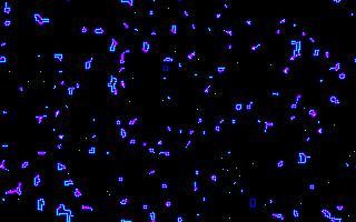
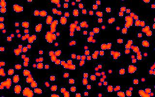
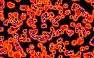
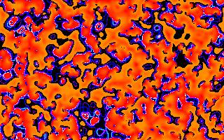
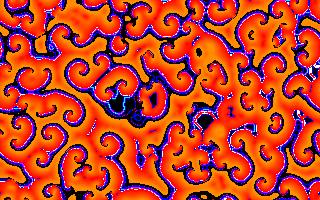
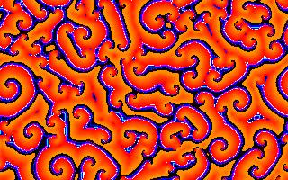
The ' process ' of a CA can lead to system states, which show an ordering, thus an ' organization ' of system elements into a definite pattern (Grid patterns, most clearly visible in 2-dimensional CA's (i.e. in CA's which have a two-dimensional cell grid, which thus looks like a checker-board)). This pattern can remain constant (steady state) or it can, together with a number of other patterns, form a cycle.
In such a CA the interaction of system elements is simulated, and these interactions can lead to self-organization of those system elements towards a coherent pattern.

In the figures we see such patterns being generated, by a 2-dimensional CA, with a rule called " Hodge ". The figures are (not immediately) successive system states (reading the figures from top to bottom). When this CA is running, the pattern is in constant motion, and reminds us strongly of the patterns we observe in a real, particular (chemical) system, called the Belousov-Zhabotinsky Reaction.

For examples of ordered, complex and chaotic CA-dynamics click HERE

back to homepage

****************